Analysis of the Impact of COVID-19 on the US Air Transport

Industry

Junhan Lin

School of Mathematical Science, Nankai University, Tianjin, China

Keywords: Time Series Analysis, Economic Recovery, Air Transport Industry.

Abstract: Public safety incidents can have widespread economic consequences, making it essential to assess their impact

and recovery patterns. This study examines the effects of COVID-19 on the U.S. air transport industry,

focusing on its post-pandemic recovery. Using time series analysis, a counterfactual forecast model based on

the U.S. air transport producer price index (PPI) is constructed to estimate industry trends unaffected by the

pandemic. The accuracy of the model is evaluated using mean absolute error (MAE) and R-squared indices,

providing a comparative analysis against actual data. The results reveal a gradual return to pre-pandemic

trends and offer insights into industry resilience. This study contributes to a broader understanding of

economic recovery dynamics and provides a methodological approach applicable to similar disruptions in

other sectors. Furthermore, the findings can inform policymakers and industry stakeholders in developing

more effective strategies for mitigating the economic impact of future crises, enhancing the adaptability and

sustainability of affected industries in the long run.

1 INTRODUCTION

In recent decades, public safety incidents have

occurred frequently. Because of their suddenness and

unpredictability, these emergency events have caused

huge losses for people all over the world. If the

emergence and development of them can be predicted

and analyzed by technical means, the damage would

be controlled (Alexander, 2002; Cutter, Boruff, &

Shirley, 2003).

Emergency time series analysis is a research

subfield contained within the field of time series

analysis, which focuses on analyzing the impact of

emergencies on the dynamic changes of time series

data, and aims to advise on public safety decisions

through analysis, modeling and forecasting (Box et

al., 2015; Wang & Ye, 2018; Hyndman &

Athanasopoulos, 2018). Given the frequent

occurrence of emergency events in recent years, this

research field has also received more attention.

In this field of emergency time series analysis,

there are many methods that are consistent with those

in time series analysis, researchers use ETS, ARIMA,

or other forecast methods to construct a forecast

model, test its performance and forecast the future

https://orcid.org/0009-0001-8760-2324

changes in the time series in research (Zhao, 2009;

Taylor, 2003; Wei, 2006).

While several studies have extensively analyzed

the macroeconomic impact of COVID-19, research

on its effects at the industry level remains relatively

limited (Bayati et al., 2025; Eichenbaum et al., 2021).

Understanding how specific industries have been

affected is crucial for developing targeted recovery

strategies and informing policy decisions. However,

there is still a lack of comprehensive studies that

assess the long-term implications of the pandemic on

individual sectors.

This research aims to study the impact of COVID-

19 on the producer price index (PPI) of the U.S. air

transportation industry and its recovery status. In the

research, the author used the ARIMA model to

forecast the dynamic changes of the PPI of the U.S.

air transportation industry without affection of the

pandemic, analyzing the recovery status of U.S. air

transportation PPI by comparing the forecast time

series with the actual.

This research is divided into four parts, the first

part is the introduction of the study, the second part is

data pre-processing and research methods, the third

Lin, J.

Analysis of the Impact of COVID-19 on the US Air Transport Industry.

DOI: 10.5220/0013698000004670

Paper published under CC license (CC BY-NC-ND 4.0)

In Proceedings of the 2nd International Conference on Data Science and Engineering (ICDSE 2025), pages 385-391

ISBN: 978-989-758-765-8

385

one is the model construction and analysis, and the

last one is the conclusion of this research.

2 DATA PRE-PROCESSING AND

METHODS

2.1 Data Collection and Description

The data of this research were obtained from the

FRED website, and the series name is "Producer Price

Index by Industry: Air Transportation(PCU481481)

". The data is provided by the U.S. Bureau of Labor

Statistics and published via the FRED website.

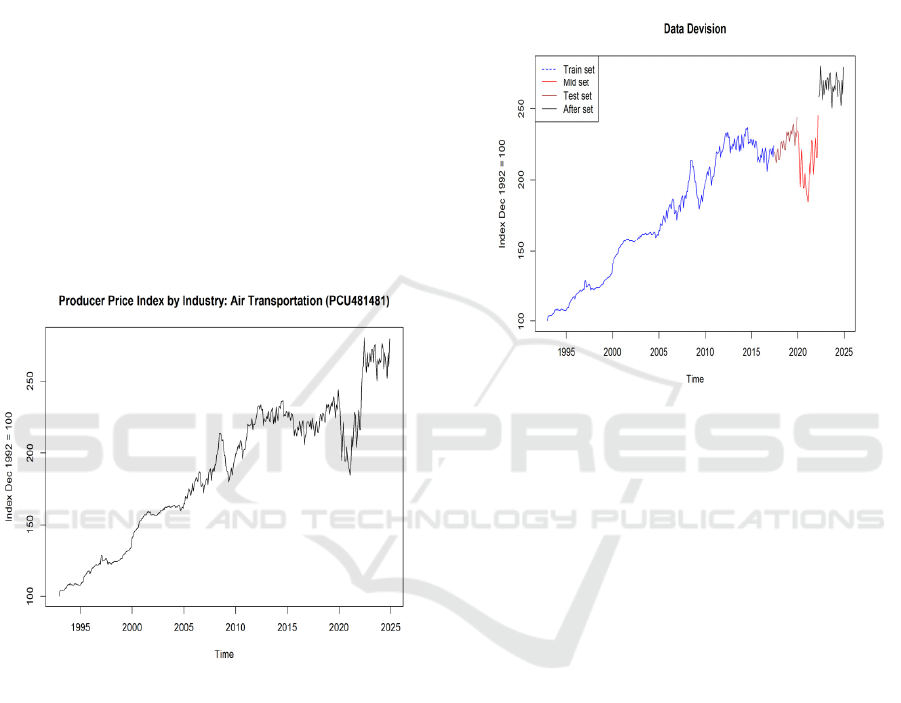
In Figure 1, the data time series shows the

monthly change in the PPI of the U.S. air

transportation industry from December 1992 to

December 2024, with the base index value 100 of

December 1992.

Figure 1: Air Transportation (PCU481481) Producer Price

Index. (Picture credit: Original)

2.2 Data Pre-processing

First, the author divides the data into two parts. Part I

is the model training and test part, data from Dec 1992

to Dec 2019, which is used to construct the

forecasting model and evaluate the performance of

the model. In this part, the author further split the data

into training and test sets. Among them, the training

set contains data from Dec 1992 to Jun 2017,

accounting for about 90\% of the Part I data, and the

test set contains about 10\% of the total Part, data

from Jul 2017 to Dec 2019.

The other part is to assess the impact of COVID-

19 on the U.S. Air Transportation Industry PPI and its

recovery status, from Jan 2020 to Dec 2024. In this

part, the time series is divided into the mid-set and the

after set, the former data from Jan 2020 to Apr 2022,

corresponding to pandemic-era data, and the latter

corresponds to post-pandemic data from May 2022 to

Dec 2024. Figure 2 shows the exact segmentation.

Figure 2: Data Division. (Picture credit: Original)

2.3 Method

2.3.1 Introduction to the ARIMA Model

A time series is a set of random variables ordered by

time, and time series analysis is a subject that studies

time series. In this subject, ARIMA is a basic model

used for forecasting and solving time series problems

with randomness, seasonality and stationarity, and it

is a basic method for handling problems in the field

of time series analysis.

1 − 𝜙



𝐵−𝜙



𝐵



−⋯−𝜙



𝐵





(

1−Φ



𝐵



−⋯−Φ



𝐵



)

(

1−𝐵−⋯−𝐵



)

(

1−𝐵



−⋯−𝐵



)

𝑦



=1+𝜃



𝐵+⋯+𝜃



𝐵





1 + Θ



𝐵



+⋯+Θ



𝐵



𝜖



(

)

where {𝑦



} is the value of the time series when

time goes to 𝑡, 𝜀



=𝑦



−𝑦



is the difference of the

time series at time 𝑡, 𝐵 is the backward shift operator,

when 𝐵 operating on 𝑦



, has the effect of shifting the

data back one period. And 𝜙, Φ, 𝜃, Θ are variable

parameters.

ICDSE 2025 - The International Conference on Data Science and Engineering

386

3 MODEL, FORECAST AND

ANALYSIS FOR PPI OF U.S.

AIR TRANSPORTATION

3.1 Testing and Processing of Data

Stationarity

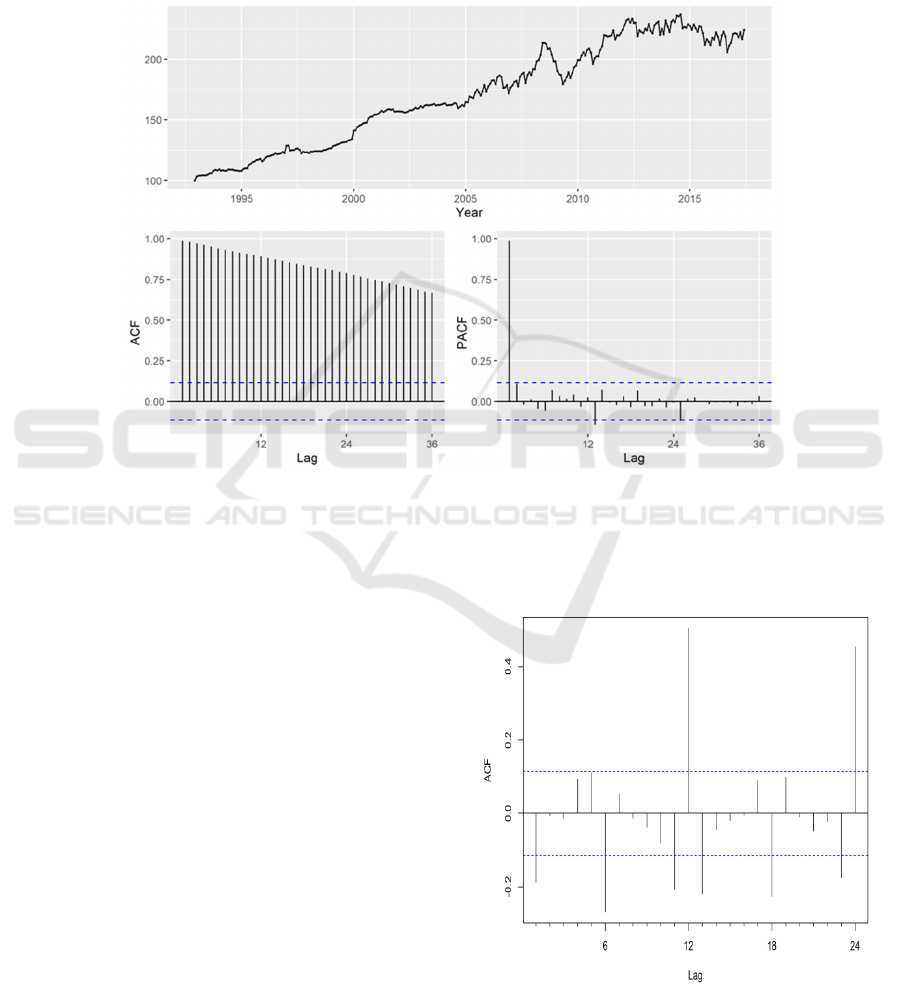
Based on the known U.S. air transportation PPI data

from December 1992 to June 2017, its time series

plot, ACF plot and PACF plot have been drawn

below(Figure 3).

Figure 1: Display of Training Set. (Picture credit: Original)

The time series plot exhibits non-stationary

transparency. Applying the Kwiatkowski-Phillips-

Schmidt-Shin (KPSS) test on the training set, the

people can find that p-value = 4.9148 much bigger

than 0.05, suggesting that the training set is non-

stationary. So seasonal and non-seasonal differencing

methods are applied on the training set to satisfy the

stationarity assumption of data.

3.2 Model Identification

According to the given non-stationary training data,

choosing the degree of difference d and D is the first

important thing. The coding above shows that the

training set is not stationary, and as the ACF plot of

the given time series sees a slow downward trend

which indicates the given time series may satisfy a

mixed time series model, Seasonal-ARIMA model\

𝐴𝑅𝐼𝑀𝐴(𝑝,𝑑,𝑞)(𝑃,𝐷,𝑄)



has been employed.

Firstly, due to the non-stationarity of the time

series, the data is made a non-seasonal difference and

found in its ACF chart that the value of lag = 12 is

very high, but the surrounding values are not so, as

shown in figures below(Figure 3, Figure 4), which

reflects that the time series has a strong seasonality

with a period of 12.

Figure 2： ACF plot of the First Difference Data. (Picture

credit: Original)

Analysis of the Impact of COVID-19 on the US Air Transport Industry

387

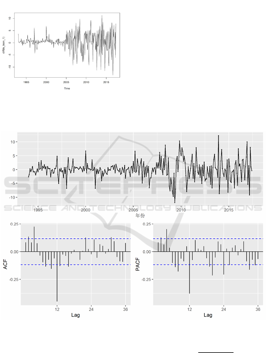
Figure 3：Plot of the First Difference Data. (Picture credit:

Original)

Therefore, it is necessary to make seasonal

differences between the different time series. At the

same time, it can be judged that the seasonal model

conforms to the MA(1) model. The KPSS test is

conducted on the series after seasonal difference

(d=1, D=1), and the p-value is 0.0172, which is lower

than 0.05, showing that the time series now is

stationary.

Finally, considering the order p of the non-

seasonal autoregressive model and the order q of the

moving average model. Figure 6 shows that the ACF

and PACF plots of this series show obvious spikes at

lag=5, and among the data with lag greater than 5,

there is no larger autocorrelation coefficient than

lag=5.

Therefore, p = 5 and q = 5 are the most appropriate

models, but after AIC testing, this paper finds that in

the binary array where p and q belong to 0 to 15, there

is no model with a lower AIC value than the model

(5,1,7), which reflects that 𝐴𝑅𝐼𝑀𝐴(5,1,7)(0,1,1)



a more consistent model.

Figure 4： Tsdisplay Plot of Seasonal and Non-seasonal Differencing Data. (Picture credit: Original)

3.3 Testing of the Model

The R-square test is the basic test index of the fit of

regression model test, which is defined by the

following formula.

𝑟



=1 −

∑(

𝑦



−𝑦





)







∑(

𝑦



−𝑦

)







(

)

ICDSE 2025 - The International Conference on Data Science and Engineering

388

Where {𝑦



} as the actual value, {𝑦



} as the

predicted value, {𝑦} is the average for {𝑦



Taking the test set data from Jul 2017 to Dec 2019

as the actual value and the predicted data of

𝐴𝑅𝐼𝑀𝐴(5,1,7)(0,1,1)



as the predicted value,

performing the R-square test and obtaining the value

0.65. Considering that the R-square attribute is

sensitive to outliers if the last outlier is removed, the

R-square value can be higher.

When choosing an increase in data value as a

positive class and a decrease as a negative class.

Precision can be expressed as 𝑃𝑟𝑒𝑐𝑖𝑠𝑖𝑜𝑛 =





where TP is True Positives, represents the number of

samples predicted by the model to be of positive class

and actually of positive class, FP is False Positives,

represents the number of samples predicted by the

model to be in the positive class but actually in the

negative class.

After calculation, it can be seen that the precision

of 𝐴𝑅𝐼𝑀𝐴(5,1,7)(0,1,1)



is 0.909, indicating the

high accuracy of forecasting models when predicting

upward movements.

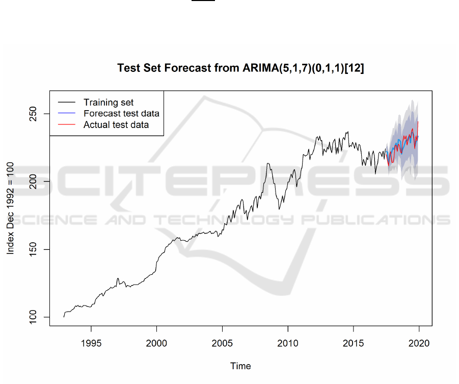
According to the high R-squared value and

Precision value of the test set, the selected forecast

model shows a high degree of fit, so that in

subsequent analysis, the model will be considered as

normal developed state of U.S. air transport PPI

without the affection of COVID-19. Below is a plot

of the predicted and actual values in the test set,

showing the high degree of fit of the forecast model.

Figure 5：Test Set Forecast from 𝐴𝑅𝐼𝑀𝐴(5,1,7)(0,1,1)



.(Picture credit: Original)

The following figure reflects the long-term

prediction of the selected model. It shows that the PPI

of the US air transportation was affected by the

epidemic from January 2020 to April 2022 (Mid set),

which was lower than the data of December 2019. At

this stage, the R-square value of the model predicted

value and the actual value is only 0.104, while the

precision of 𝐴𝑅𝐼𝑀𝐴(5,1,7)(0,1,1)



is declined to

0.636, indicating that the U.S. air transport PPI

suffered a huge impact by COVID-19 in the first half

period, and then entered a state of gradual recovery in

the second half of the period.

Analysis of the Impact of COVID-19 on the US Air Transport Industry

389

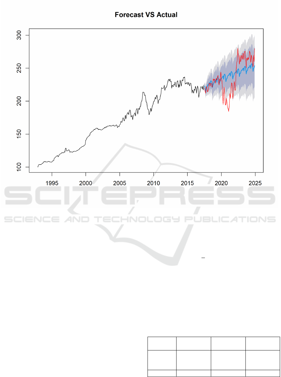
Figure 6: Plot pf Forecast Data and Actual Data. (Picture credit: Original)

Besides, in the After period (from May 2022 to

Dec 2024), the actual data of U.S. air transport PPI is

bigger than the forecast one due to a sharp increase in

early 2022, then the actual data shows a downward

trend until the latest data. The former may based on

the rise in labor prices caused by revenge travel after

the epidemic, while the latter trend reflects that the

U.S. air transport industry gradually is getting rid of

the impact of the epidemic and returning to normal.

However, Over the entire period, the data do not

return to normal compared to the Mid set, since the

R-squared value is 0.109 and the precision of the data

is 0.667, which are just a little bigger than the Mid set.

When the after set is divided into three equal

parts(from Apr 2022 to Feb 2023, May 2023 to Jan

2024 and Feb 2024 to Dec 2024), their R-squared

values and Mean Absolute Error(MAE) values

indicate that the U.S. air transport PPI is getting back

to normal, and will become normal soon in early

2025.

Mean Absolute Error (MAE) is a statistical

measure used to evaluate the average magnitude of

errors between predicted and actual values, without

considering the direction of the errors. The formula

for MAE is:

𝑀𝐴𝐸 =

𝑛

|𝑦







−𝑦



|#(3)

Where n is the number of observations, {𝑦



} as the

actual value and {𝑦



} as the predicted value. The

following table shows the R-squared values and MAE

values of each interval time series, the MAE is getting

smaller and the R-squared is getting bigger as time

goes by. Table 1 shows the Results.

Table 1：Experiment Results

Apr 2022 to

Feb 2023

May 2023

to Jan 2024

Feb 2024 to

Dec 2024

R-

squared

value

-20.04126 -16.34049 -9.505967

MAE 29.42327 27.3092 24.06513

ICDSE 2025 - The International Conference on Data Science and Engineering

390

4 CONCLUSIONS

In this study, the author used the pre-epidemic data of

U.S. air transport PPI and applied the ARIMA

method to construct a prediction model with a high

fit, which is not affected by the epidemic. By

comparing selected models with actual data, the

researcher quantified the impact of the pandemic on

the data, analyzed the possible causes of the dynamic

change of data and made a conclusion that the U.S.

air transport industry will get back to normal soon, the

government should opt for conservative incentives to

finely adjust the air transport industry.

However, due to the incompleteness of data, the

author can not verify the correctness of the conclusion

for the time being. Besides, this research did not delve

into the impact of the pandemic on the changes in

addition and deletion in data, as the precision declined

from about 0.9 to 0.6, but the study does not find its

reason.

Finally, it is hoped that this study will play a role

in establishing the analysis system of the impact of

public safety incidents on the industry, or in helping

the public safety decision.

REFERENCES

Alexander, D. E. (2002). Principles of emergency planning

and management. oxford university press.

Cutter, S. L., Boruff, B. J., & Shirley, W. L. (2003). Social

vulnerability to environmental hazards. Social science

quarterly, 84(2), 242-261.

Box, G. E., Jenkins, G. M., Reinsel, G. C., & Ljung, G. M.

(2015). Time series analysis: forecasting and control.

John Wiley & Sons.

Wang, Z., & Ye, X. (2018). Social media analytics for

natural disaster management. International Journal of

Geographical Information Science, 32(1), 49-72.

Hyndman, R. J., & Athanasopoulos, G. (2018). Forecasting:

principles and practice. OTexts.

Zhao, G. (2009). Research on stock price trend prediction

based on time series analysis (Doctoral dissertation,

Xiamen University). Xiamen University.

Taylor, J. W. (2003). Exponential smoothing with a damped

multiplicative trend. International journal of

Forecasting, 19(4), 715-725.

Wei, W. W. (2006). Univariate and Multivariate methods.

TIME SERIES ANALYSIS.

Bayati, M., Lotfi, F., Bayati, M., & Goudarzi, Z. (2025).

The effect of Covid-19 pandemic on the primary health

care utilization and cost: an interrupted time series

analysis. Cost Effectiveness and Resource Allocation,

23(1), 1-7.

Eichenbaum, M. S., Rebelo, S., & Trabandt, M. (2021). The

macroeconomics of epidemics. The Review of

Financial Studies, 34(11), 5149-5187.

Analysis of the Impact of COVID-19 on the US Air Transport Industry

391