
Forecast USD/RMB Exchange Rate and Fitting Comparison Based on
Three Methods
Sitong Song
a
Statistics and Mathematics College, Inner Mongolia University of Finance and Economics, Hohhot, Inner Mongolia
Autonomous Region, China
Keywords: ARIMA, ETS, SMA, Exchange Rate Forecasting.
Abstract: In light of the current complex and volatile international landscape, continuously updated exchange rate
forecasts are indispensable. Accurate exchange rate forecasts enable enterprises to mitigate trade risks and
optimize investment decisions, assist financial institutions in risk management, and support policy
formulation. Furthermore, they provide robust support for macroeconomic policymakers, helping to maintain
exchange rate stability, balance international payments, and foster steady economic growth, which holds
significant importance across all economic levels. In this paper, through Auto-Regressive Integrated Moving
Average Model (ARIMA), Error-Trend-Seasonal (ETS) and Simple Moving Average (SMA) traditional time
series models forecast the next 10 steps (one step every five consecutive working days) based on the
USD/RMB exchange rate in 2022-2025. The result is compared with the actual value pair. In this study, the
Akaike Information Criterion (AIC) and Bayesian Information Criterion (BIC) are employed for model
selection when utilizing ARIMA, ETS, and SMA models. The model's performance was assessed using Root
Mean Squared Error (RMSE) and residual P-values. Given the volatile international situation, updated
exchange rate forecasts are needed. Accurate exchange rate forecasts enable enterprises to mitigate trade risks
and optimize investment decisions, assist financial institutions in risk management, and support policy
formulation.
1 INTRODUCTION
Over the past few decades, due directly to the factors
mentioned above, there has been a significant
acceleration in the expansion of forex exchange
markets driven by increased cross-border capital
flows (de Paula, Ferrari-Filho, & Gomes, 2013). A
number of economic indices exist for this market but
perhaps the most crucial is exchange rates (Baffour et
al., 2019). Exchange rate forecast is a very important
part of the foreign exchange market, and it plays a
very important role in the external development of
enterprises and social and economic development and
provides an important evaluation index. Previously,
many experts and scholars have used traditional time
series models to fit together and accurately updated
and adjusted the model to make it more suitable for
today's global situation. Even though conventional
models like the ARIMA are regarded as efficient
methods, they demand both stationary time series and
a
https://orcid.org/0009-0006-6825-1895
non - stationary time series that have been
appropriately transformed to become stationary
(Cappello et al., 2025). The ARIMA model was used
to stabilize the difference of the data and then proved
to reach the predictable stage by different test
standards. The model parameters were adjusted and
fitted, and the rationality of this model for short-term
exchange rate prediction was obtained. Using the
time series model to forecast the exchange rate over a
short period is beneficial to the trade development of
import and export enterprises and can provide
investment basis for international investors (Jiang &
Liu, 2022). The remaining two models underwent the
best process via steps similar to the first one. In this
study, the core objective is to identify the most
premier prediction model for short - term time series.
This is achieved by juxtaposing the three models
against the actual values. Initially, the paper
meticulously preprocesses the data and assesses its
fitting potential. Subsequently, distinct parameters
Song, S.
Forecast USD/RMB Exchange Rate and Fitting Comparison Based on Three Methods.
DOI: 10.5220/0013697800004670
Paper published under CC license (CC BY-NC-ND 4.0)
In Proceedings of the 2nd International Conference on Data Science and Engineering (ICDSE 2025), pages 379-384
ISBN: 978-989-758-765-8
Proceedings Copyright © 2025 by SCITEPRESS – Science and Technology Publications, Lda.
379
within different models are adjusted. Eventually, the
goodness of each model is evaluated from two diverse
dimensions, leading to a well - founded conclusion.
2 DATA AND METHOD
2.1 Data Collection and Description
This study acquires its data from China Money
Network by visiting the website and downloading the
data. This dataset includes 728 USD/RMB exchange
rate data from January 1, 2022 to January 1, 2025.
The data set is grouped by weekdays, that is, data
points are grouped by every five consecutive working
days. The specific sample information is shown in
Table 1:
Table 1: Sample description.
Statistical Index
Numerical
Value
Remark
Number of Data
Points
728
Daily data, spanning
two years
Exchange Rate
Minimum
6.3014
44621
Exchange Rate
Maximum
7.2258
45107
Average
Exchange Rate
6.85
Based on the data
Data Frequency
Everyday
One data point per
business day
Data Integrity
Integrity
No missing value
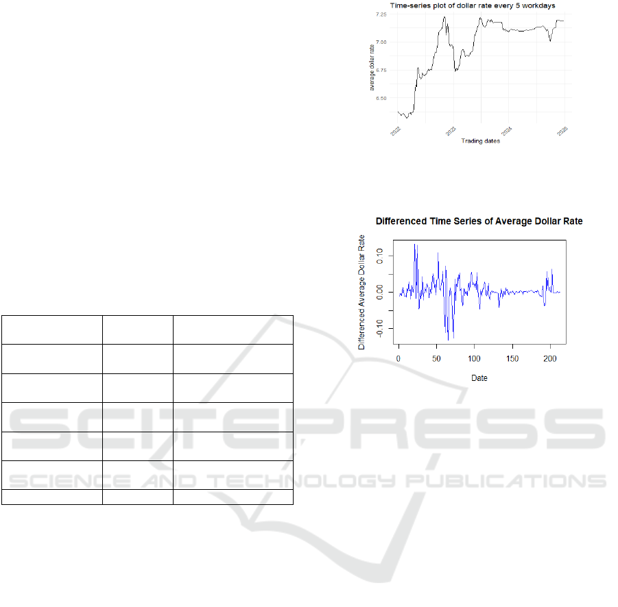
2.2 Data Pre-processing
Through data cleaning, the error value and missing
value in the data are eliminated. In this paper, RStudio
software was used to analyse the data, and the
samples were drawn into a time series chart (Figure
1). It can be found that since the epidemic had just
ended at this time, economic activities and market
environment had not completely returned to the stable
state, so there was a sharp rise in the first period and
a sharp decline in the subsequent data, and the
subsequent data also fluctuated. The differential data
(Figure 2) are stable and eliminate long-term trends.
This represents an expansion of the Autoregressive
Moving Average Process applicable to time series
processes lacking stationarity. In this approach, the
data is subjected to a transformation so as to convert
the process into a stationary one (Marcy, 2021).
Figure 1: Timing diagram of original data (Picture credit:
Original)
Figure 2: Stationary sequence diagram after difference
(Picture credit: Original).
2.3 Auto-Regressive Integrated Moving
Average Model(ARIMA)Model
Principle
ARIMA is widely used in time series prediction
analysis. Its essence aims to transform non-stationary
time series into stationary ones through difference
operation, and then build ARIMA model and perform
prediction analysis. The ARIMA model, short for
moving average with auto-regressive integration is
usually represented as ARIMA. In this model, “p”
represents the order of the autoregressive part, “d”
indicates the level of differencing necessary, and “q”
stands for the order of the moving average part (Chen
et al., 2023). The basic structure of the model is
shown in formula (1), formula (2) and formula (3):
Where
is the polynomial of the moving
smoothness coefficient,
is the polynomial of
ICDSE 2025 - The International Conference on Data Science and Engineering
380
the autoregressive coefficient, and {
} is the zero-
mean white noise sequence (Sun & Cheng, 2016). In
the analysis of time series, autocorrelation and partial
autocorrelation tests are carried out for the difference
series, and the orders of autoregression (p) and
moving average (q) within the ARIMA model are
preliminarily inferred. Then, The Akaike Information
Criterion (AIC), Bayesian Information Criterion (BIC)
and Root Mean Squared Error (RMSE) were
comprehensively used to identify and determine the
ARIMA model more accurately, and the most
suitable ARIMA model was selected. After the model
is selected, the fitting performance of the model is
evaluated by its residual sequence and correlation
coefficient. If the remainder sequence is similar to the
white noise and the correlation coefficient is within a
reasonable range, it indicates that the model has a
good fitting effect on the data. If not, model flaws
exist; optimize. ARIMA forecasts, and real -
predicted value comparison gauges its practical
reliability.
2.4 Error-Trend-Seasonal(ETS)
Model Principle
Exponential smoothing method is to use the average
based on weighted values of the actual observed
amounts of the series to prognosticated the projected
value, the latest data in the series is multiplied by a
most substantial weight, and the data over the long
haul is added with a lesser weight (Shao et al., 2021).
TS model is a smoothing method, which is widely
used in processing time series data with seasonality
and trend (Li et al., 2025). Exponential smoothing
uses error, trend, seasonal params. ETS auto - selects,
adjusts, and evaluates to find best - performing model.
In the process of model selection, the best-fit model
is chosen relying on the minimum values of AIC, BIC
and RMSE. The P-value of the residual is tested by
Ljung-box Q to determine whether the residual is
white noise.
2.5 Simple Moving Average(SMA)
Model Principle
Moving average method is a method to calculate the
average containing a certain number of items to
reflect the changing trend of time series. The details
are shown in formula (4):
,
Where
is the moving average of the period
and represents the quantity of moving average
items.
The prediction method is shown in formula (5):
The period’s moving average is used as the
predictive value of period . By checking the P-
value of the residual, the people can judge whether
the residual is white noise. In general, the predicted
values of subsequent periods can be calculated
accordingly. Error accumulation causes larger errors
later; SMA suits one - period - ahead forecasts.
3 RESULTS AND DISCUSSION
3.1 ARIMA Model
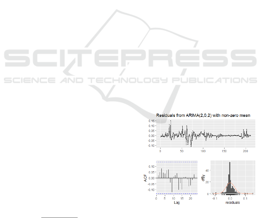
3.1.1 Model Fitting
Autocorrelation Function (ACF) and Partial
Autocorrelation Function (PACF) of data after first-
order difference are shown in Figure 3. This article
uses RStudio to try different parameter combinations,
as shown in Table 2, and finally determines that
ARIMA (2,1,2) is optimal. AIC, BIC and RMSE of
ARIMA (2,1,2) are all the smallest. The residual P
value exceeded 0.05. At this time, the data of
logarithmic first-order difference have excellent
performance in AIC, BIC and RMSE detection. If the
residual is white noise, most of the information parts
of the model have been extracted and can be fitted.
Figure 3: ARIMA (2,1,2) residual test (Picture credit:
Original).
Forecast USD/RMB Exchange Rate and Fitting Comparison Based on Three Methods
381
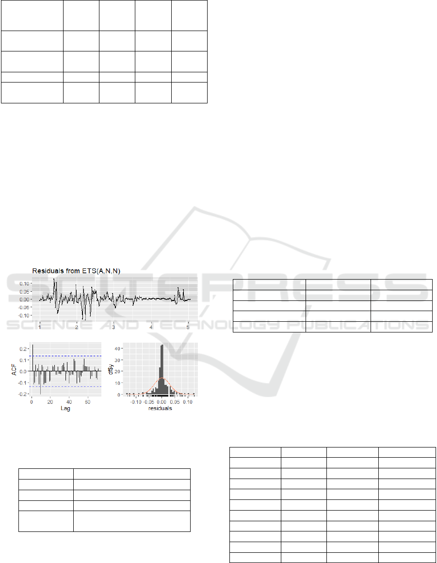
Table 2: Comparison of different parameters.
Metric
ARIM
A
(2,1,2)
ARIM
A
(3,1,4)
ARIM
A
(2.1.3)
ARIM
A
(3,1,3)
AIC
-
915.21
-
904.32
-
905.11
-
904.37
BIC
-
895.07
-
-
-
RMSE
0.0271
0.0270
0.0272
0.0271
Residual p-
value
0.2045
0.1378
0.1435
0.1562
3.2 ETS Model
3.2.1 Model Fitting
In this paper, RStudio was used to try to predict
ETS. Different parameter combinations were shown
in Table 3, and it was found that ETS (A, N, N) was
the best. The residual P value of ETS (A, N, N) is
0.0506 and greater than 0.05, and the residual is white
noise. The test result of the residual is presented in
Figure 4, then the model has extracted most of the
information. Model AIC, BIC are small. After the
model's convergence is judged, it is found to fit well.
Figure 4: ETS (A, N, N) residuals test (Picture credit:
Original).
Table 3: ETS (A, N, N) Each detection index.
ETS (A, N, N)
AIC
-350.5486
BIC
-340.4789
RMSE
0.0176
Residuals p-
value
0.05063
3.3 SMA Model
3.3.1 Model Fitting
In this paper, RStudio was used to attempt SMA
prediction, and it was found that the residual error of
the SMA model after extracting information was
0.1787, greater than 0.05, and the residual error was
white noise, so the model had extracted most of the
information parts. When
test is carried out, it
reaches 1, which proves that the model has a good
fitting effect. By judging the convergence and
divergence of the model, it is found that it is
convergent, so it can be fitted.
3.4 Experimental Result
3.4.1 Comparison Model Parameter
In the fitting of ARIMA model and ETS model, AIC,
BIC and RMSE indictors were applied to assess the
feasibility of the model. In the comparison of model
goodness, the above indexes are first used for
selection.
Table 4: Comparison of ARIMA and ETS model goodness.
ARIMA (2,1,2)
ETS (A, N, N)
AIC
-915.21
-350.5486
BIC
895.07
-340.4789
RMSE
0.0271
0.0176
Residuals p-value
0.2045
0.05063
It is obvious that from Table 4 that the AIC, BIC
and RMSE of ARIMA (2,1,2) are smaller, so the
fitting influence of ARIMA (2,1,2) is better.
3.4.2 Contrast Error Value
In the ARIMA (2,1,2) forecast:
Table5: ARIMA (2,1,2) Model Error.
Date
Forecast
TRUE
Error
2025,1
7.1897
7.1878
0.0019
2025,2
7.1933
7.1886
0.0047
2025,3
7.1923
7.1882
0.0041
2025,4
7.1917
7.1826
0.0091
2025,5
7.1925
7.1703
0.0222
2025,6
7.1922
7.1698
0.0224
2025,7
7.1921
7.1693
0.0228
2025,8
7.1923
7.1699
0.0224
2025,9
7.1922
7.1713
0.0209
2025,10
7.1922
7.1704
0.0218
ICDSE 2025 - The International Conference on Data Science and Engineering
382
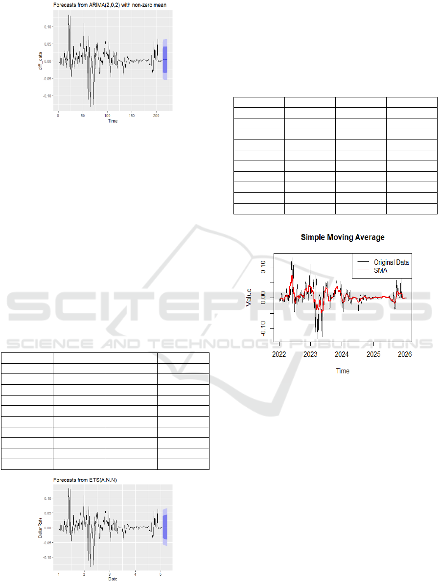
Figure 5: ARIMA (2,1,2) Forecast Graph (Picture credit:
Original).
It is evident that Table 5 that the error is inside the
range of [0.0019,0.0228]. After calculation, the
average relative error is 0.01523, which is within the
normal range and the predicted value is too large. It
shows that it is feasible to use ARIMA model to
predicting RMB exchange rate, and the overall
prediction effect is good, which is capable of
effectively predict the future currency rate trend. In
addition, as the forecast time elapses, the deviation
among the forecast value and the factual value has a
tendency to expand, so this simulation is better
adapted to short-term exchange rate prediction (Zhu
& Hu, 2019). The forecast trend is shown in Figure 5.
In ETS(A,N,N) forecast:
Table 6: ETS (A, N, N) Model Error.
Date
Forecast
TRUE
Error
2025,1
7.1906
7.1878
0.0028
2025,2
7.1928
7.1886
0.0042
2025,3
7.195
7.1882
0.0068
2025,4
7.1971
7.1826
0.0145
2025,5
7.1993
7.1703
0.0290
2025,6
7.2015
7.1698
0.0317
2025,7
7.2037
7.1693
0.0344
2025,8
7.2059
7.1699
0.0360
2025,9
7.2081
7.1713
0.0368
2025,10
7.2102
7.1704
0.0398
Figure 6: ETS (A, N, N) Forecast Graph (Picture credit:
Original).
As is evident from Table 6 that the error falls
within the scope of [0.0028,0.0398]. After calculation,
the average relative error is 0.0236, which is within
the normal range and the predicted value is too large.
The specific forecast trend is shown in Figure 6.
In the SMA forecast:
Table 7: SMA Model Error.
Date
Forecast
TRUE
Error
2025,1
6.7919
7.1878
-0.3959
2025,2
6.9383
7.1886
-0.2503
2025,3
6.7388
7.1882
-0.4494
2025,4
7.0478
7.1826
-0.1348
2025,5
7.0204
7.1703
-0.1499
2025,6
6.9553
7.1698
-0.2145
2025,7
6.8683
7.1693
-0.3010
2025,8
6.7866
7.1699
-0.3833
2025,9
6.9466
7.1713
-0.2247
2025,10
6.9984
7.1704
-0.1720
Figure 7: SMA Comparison of model prediction and
original data (Picture credit: Original).
Table 7 reveals that the error is in the bounds of
[0.1348,0.4494]. Avg. rel. error (0.26758) exceeds
norm; predictions low. The comparison between the
specific predicted value and model fitting is shown in
Figure 7.
Among simple time - series models for
USD/RMB rate, ARIMA shows top - notch fit. It's
effective for stationary data, assuming linear future
value determination. However, many real-world time
series data exhibit complex nonlinear patterns that
ARIMA cannot model effectively (Zhang, 2023).
Simple moving average and exponential moving
average are two standard technical analysis
techniques (Billah et al., 2024). Predictions lose
accuracy as lead time increases (Tian, 2017).
Forecast USD/RMB Exchange Rate and Fitting Comparison Based on Three Methods
383

4 CONCLUSIONS
By comparing the estimated value and the value
observed in practice and drawing the time series
graph, this paper find that the ARIMA model has the
best fitting effect on the USD/RMB exchange rate. In
this paper, three traditional time series models of
ARIMA, ETS and SMA were used to predict the
USD/RMB exchange rate in the next 10 steps, and
then the goodness of fit of the three models was
evaluated through two dimensions. The first
dimension is that the results of ARIMA (2,1,2) model
are better by comparing AIC, BIC, RMSE and
residual P-value. The second dimension shows that
ARIMA (2,1,2) has the smallest error by comparing
the predicted value with the actual value, followed by
ETS (A, N, N), and finally SMA, and all three models
are within the normal error range. The limitation of
this paper is that the traditional time series model used
in this paper will lead to fitting errors when predicting
exchange rates with large fluctuations and
randomness. The traditional statistical model has the
disadvantage of being rigid, and the results obtained
will not have good fitting effect when the original
data does not meet some assumptions. Using the
traditional time series model to forecast the exchange
rate can make the innovation foundation more solid,
the thinking clearer, and the innovation more accurate
exchange rate prediction model. It can also be
concluded from the above methods that traditional
time series models like ARIMA model are suitable
for short-term forecasting and have higher accuracy
than long-term forecasting.
REFERENCES
Baffour, A. A., Feng, J., & Taylor, E. K. (2019). A hybrid
artificial neural network - GJR modeling approach to
forecasting currency exchange rate volatility.
Neurocomputing, 365, 285-301.
https://doi.org/10.1016/j.neucom.2019.07.088
Cappello, C., Congedi, A., De Iaco, S., & Mariella, L.
(2025). Traditional prediction techniques and machine
learning approaches for financial time series analysis.
Mathematics, 13(3), 537.
https://doi.org/10.3390/math13030537
Chen, Y. H., Bhutta, M. S., Abubakar, M., Xiao, D. T.,
Almasoudi, F. M., Naeem, H., & Faheem, M. (2023).
Evaluation of machine learning models for smart grid
parameters: Performance analysis of ARIMA and Bi-
LSTM. Sustainability, 15(11), 8555.
https://doi.org/10.3390/su15118555
de Paula, L. F., Ferrari-Filho, F., & Gomes, A. M. (2013).
Capital flows, international imbalances and economic
policies in Latin America. In Economic Policies,
Governance and the New Economics (pp. 209-248).
London: Palgrave Macmillan UK.
Jiang, Q., & Liu, Y. W. (2022). Prediction of US dollar
exchange rate based on ARIMA model. Economic
Research Guide, (20), 69-71.
Li, Y. L., Lin, S., Ni, Y. T., Yao, K. Y., & Li, Y. F. (2025).
Time-series forecasting of electric power material
demand based on the "STL+ARIMA" model. Internet
Weekly, (02).
Marcy, J. (2021). Time series regression and intervention
analysis [Doctoral dissertation, College of Charleston].
ProQuest Dissertations and Theses Global. (28866113)
Shao, Y. Q., Liu, H., Li, C. X., Meng, X. W., Li, L., Wang,
X., & Wu, Q. H. (2021). Application of SARIMA and
ETS models in predicting the incidence trend of
hemorrhagic fever with renal syndrome in Hunan
Province. Chinese Journal of Health Statistics, XX(XX),
XX-XX. https://doi.org/10.3969/j.issn.1002-
3674.2021.02.012
Sun, P., & Cheng, C. M. (2016). Research on exchange rate
forecasting based on ARIMA model: Taking the US
Dollar - RMB exchange rate as an example. Journal of
Liaoning University of Technology (Social Science
Edition), 18(6), 20-23.
https://doi.org/10.15916/j.issn1674-327x.2016.06.006
Zhu, J. M., & Hu, L. Y. (2019). Comparative analysis of
RMB exchange rate forecast based on ARIMA and BP
neural network——Take the exchange rate of US dollar
to RMB as an example. Journal of Chongqing
University of Technology (Natural Science), 33(5),
207-212. https://doi.org/10.3969/j.issn.1674-
8425(z).2019.05.032
Zhang, P. L. (2023). Research on Exchange Rate
Forecasting Based on Deep Learning under the
Influence of US Policies. Journal of Zhongnan
University of Economics and Law (Master's Thesis),
2023(01). DOI: 10.27660/d.cnki.gzczu.2021.000320
Billah, M. M., Sultana, A., Bhuiyan, F., & Kaosar, M. G.
(2024). Stock price prediction: comparison of different
moving average techniques using deep learning model.
Neural Computing and Applications, 36(10), 5861–
5871. https://doi.org/10.1007/s00521-023-09369-0
Tian, Z. W. (2017). Research on Time - Series Analysis
Methods and Their Application in Sino - US Exchange
Rate Forecasting. Journal of Dalian University of
Technology (Master's Thesis), 2017(03).
ICDSE 2025 - The International Conference on Data Science and Engineering
384
