A Convexity-Dependent Two-Phase Training Algorithm for Deep Neural

Networks

Tomas Hrycej

1†

, Bernhard Bermeitinger

2† a

, Massimo Pavone

1‡

, G

otz-Henrik Wiegand

1† b

and

Siegfried Handschuh

1† c

Institute of Computer Science, University of St.Gallen (HSG), St.Gallen, Switzerland

Institute of Computer Science in Vorarlberg, University of St. Gallen (HSG), Dornbirn, Austria

ﬁ ﬁ

Keywords:

Conjugate Gradient, Convexity, Adam, Computer Vision, Vision Transformer.

Abstract:

The key task of machine learning is to minimize the loss function that measures the model ﬁt to the training

data. The numerical methods to do this efﬁciently depend on the properties of the loss function. The most

decisive among these properties is the convexity or non-convexity of the loss function. The fact that the loss

function can have, and frequently has, non-convex regions has led to a widespread commitment to non-convex

methods such as Adam. However, a local minimum implies that, in some environment around it, the function

is convex. In this environment, second-order minimizing methods such as the Conjugate Gradient (CG) give

a guaranteed superlinear convergence. We propose a novel framework grounded in the hypothesis that loss

functions in real-world tasks swap from initial non-convexity to convexity towards the optimum — a property

we leverage to design an innovative two-phase optimization algorithm. The presented algorithm detects the

swap point by observing the gradient norm dependence on the loss. In these regions, non-convex (Adam)

and convex (CG) algorithms are used, respectively. Computing experiments conﬁrm the hypothesis that this

simple convexity structure is frequent enough to be practically exploited to substantially improve convergence

and accuracy.

1 INTRODUCTION

Fitting model parameters to training data is the fun-

damental task of Machine Learning (ML) with pa-

rameterized models. The sizes of the models have

experienced extraordinary growth, recently reaching

hundreds of billions. This makes clear that the ef-

ﬁciency of the optimization algorithm is of key im-

portance. The optimization consists of minimizing an

appropriate loss criterion such as Categorical Cross-

Entropy (CCE), Mean Squared Error (MSE), or many

other variants. These criteria are multidimensional

functions of all model parameters. From the view-

point of solvability, there are three basic classes of un-

constrained minimization tasks according to the char-

acteristics of the minimized function:

1. Convex functions

2. Non-convex functions with a single local mini-

mum (which is also a global minimum)

https://orcid.org/0000-0002-2524-1850

https://orcid.org/0009-0009-0392-056X

https://orcid.org/0000-0002-6195-9034

3. Non-convex functions with multiple local minima

Non-convex functions are frequently referred to as

a single group in the ML literature. This aggrega-

tion shadows a signiﬁcant difference. In practical

terms and for typical numbers of trainable parame-

ters of current models, global minimization of a gen-

eral function with multiple local minima is infeasi-

ble (see Section 2). By contrast, gradient descent

can practically minimize non-convex functions with

a single local minimum. Every descending path will

reach the minimum with certainty if it is not trapped

in singularities. For convex loss functions, the odds

are even better. The classical theory of numerical op-

timization provides theoretically founded algorithms

with a guaranteed convergence speed, also referenced

in Section 2.

From the viewpoint of this problem classiﬁca-

tion, it is well known that loss functions with popu-

lar nonlinear models can possess multiple local min-

ima, and thus count to the last class mentioned. Some

of these minima are equivalent (such as those arising

through permutations of hidden-layer units), but oth-

ers may not. So, the paradoxical situation concern-

Hrycej, T., Bermeitinger, B., Pavone, M., Wiegand, G.-H. and Handschuh, S.

A Convexity-Dependent Two-Phase Training Algorithm for Deep Neural Networks.

DOI: 10.5220/0013696100004000

Paper published under CC license (CC BY-NC-ND 4.0)

In Proceedings of the 17th International Joint Conference on Knowledge Discovery, Knowledge Engineering and Knowledge Management (IC3K 2025) - Volume 1: KDIR, pages 78-86

ing the training of nonlinear models is that methods

are used that almost certainly cannot solve the prob-

lem of ﬁnding a global minimum. The implicit as-

sumption is that the existence of multiple minima can

be neglected in the hope that the concretely obtained

local minimum is sufﬁciently suitable for the appli-

cation. The positive experience with many excellent

real models seems to justify this assumption. What

remains is distinguishing between two former basic

classes: convex functions and non-convex functions

with a single minimum (further referred to simply as

non-convex).

The fact that the loss functions of popular ar-

chitectures are potentially non-convex has led to the

widespread classiﬁcation of these loss functions as

non-convex. However, from a theoretical viewpoint,

the loss function is certainly convex in some environ-

ment of the local minimum. This axiomatically re-

sults from the deﬁnition of a local minimum of any

smooth function L(x) by the gradient being zero:

∇L(x) = 0 (1)

and the Hessian

H(x) = ∇

L(x) (2)

being positive deﬁnite, i.e., having positive eigenval-

ues. There, convex minimization algorithms are cer-

tainly worth using. This guaranteed convex region

can optionally be — and frequently is — surrounded

by a non-convex region.

From this point of view, the key question for algo-

rithm choice is where the loss function is convex and

where not. Although it is known that, in general, there

may be an arbitrary patchwork of convex and non-

convex subregions, a simpler, while not universally

valid, assumption may exist that covers typical model

architectures and application tasks. One such assump-

tion is formulated in Section 3. In the next step, we

will propose the appropriate optimization procedure

accordingly (Section 4). If an assumption about a typ-

ical distribution of convexity is tentatively adopted,

it is crucial to check how frequently this assumption

applies in the spectrum of application problems. Al-

though an extensive survey is not feasible due to re-

source limitations, experiments with a variety of typ-

ical architectures (with a focus on a Transformer and

some of its simpliﬁed derivatives) are performed and

reviewed to determine the validity of the assumption

and the efﬁciency effect of optimization (Section 5).

2 RELATED WORK

The alleged infeasibility of minimizing functions with

multiple local minima is based on algorithms avail-

able after decades of intensive research. Heuristics,

such as momentum-based extensions of the gradient

method, alleviate this problem by possibly surmount-

ing barriers between individual attractors. Still, there

is no guarantee (and also no acceptable probability)

of reaching the global minimum in a ﬁnite time, since

the number of attractors and boundaries between them

is too large. Similarly, methods based on annealing or

relaxation (Metropolis et al., 1953; Kirkpatrick et al.,

1983) show asymptotical convergence in probability,

but the time to reach some probabilistic bounds is

by far unacceptable. Algorithms claiming complete

coverage of the parameter space, like those based on

Lipschitz constant bounds, or so-called clustering and

Bayesian methods such as (Rinnooy Kan and Timmer,

1987; Mockus et al., 1997) are appropriate for small

parameter set sizes less than ten.

By contrast, for non-convex functions with a sin-

gle local minimum, every descending path will reach

the minimum with certainty if not trapped in singu-

larities. Today’s algorithms, such as Adam (Kingma

and Ba, 2015), focus on efﬁciency in following the

descending path. There are convergence statements,

for example, by (Fotopoulos et al., 2024; Chen et al.,

2022). An interesting proposal for transforming a

non-convex unconstrained loss function to a convex

one with constraints is by (Ergen and Pilanci, 2023).

However, this approach applies only to neural net-

works with one hidden layer and the ReLU acti-

vation function. A good option for covering both

non-convex and convex regions would be second-

order algorithms with adaptive reaction to local non-

convexity, such as some variants of the Levenberg-

Marquardt algorithm (Levenberg, 1944; Press et al.,

1992). This algorithm is speciﬁc for least-squares

minimization. It entertains a kind of “convexity

weight” of deciding between a steepest gradient step

and the step towards the estimated quadratic mini-

mum. Unfortunately, the algorithm requires storing

an estimate of the Hessian, which grows quadrati-

cally in the number of parameters, which makes it

clearly infeasible for billions of parameters, even if

using sparse Hessian concepts.

For convex loss functions, a numerical algorithm

with a guaranteed convergence speed could be nonlin-

ear conjugate gradient method (Fletcher and Reeves,

1964) and (Polak and Ribi

ere, 1969). Both versions

and their implementations are explained in (Press

et al., 1992). They exploit the fact that convex func-

tions can both be approximated quadratically. This

quadratic approximation has an explicit minimum

whose existence can be used to approach the non-

quadratic but convex function minimum iteratively,

with the guarantee of superlinear convergence.

A Convexity-Dependent Two-Phase Training Algorithm for Deep Neural Networks

3 CONVEX AND NON-CONVEX

REGIONS OF LOSS

FUNCTIONS

In this section, the hypothesis will be pursued that the

following constellation characterizes the typical case:

There is a convex region around the minimum, sur-

rounded by a non-convex region. We are aware that

this hypothesis will not apply to arbitrary tasks. How-

ever, if this were frequently the case in typical appli-

cations, it could be exploited for a dedicated use of

ﬁrst- and second-order algorithms, respectively.

A pictorial representation of the situation is given

in Figure 1 showing the dependence of MSE on the

scaling parameter p for a set of ﬁve random tasks with

a single nonlinear layer tanh model (with 100 units)

y(x) =

∑

tanh(px) (3)

and its square loss

L(x) =



y(x) − r



(4)

with reference values r of the output y randomly

drawn from (0, 1). The set is generated for randomly

selected input arguments x from (−0.5, 0.5). Convex-

ity around the minimum and non-convexity at margin

areas can be observed.

A different view of the same ﬁve random tasks is

the dependence of gradient norm on the loss, as de-

picted in Figure 2. The gradient norm is trivial in the

one-dimensional case: it is the absolute value of the

derivative. During optimization, the loss on the x-axis

decreases (from the right to the left). The gradient

norm (the y-axis) ﬁrst increases (the non-convex re-

gion) and then decreases (the convex region) - this

pattern can be observed for all ﬁve tasks. The two

branches per task correspond to the different paths to

the minimum (starting at the left or at the right mar-

gin, respectively, in Figure 1). It should be noted that

there is no guarantee for this simple convexity pat-

tern. Our hypothesis is that this pattern is frequently

encountered and is not universally valid.

In the multidimensional parameter space, vertical

cross-sections of a convex function are also convex

so that the property of diminishing gradient norm is

retained. This is also the case for steepest gradient

paths, such as that given in the 2D plot of Figure 3; the

level curves become successively less dense along the

path. Of course, with an inappropriate step size, the

optimization trajectory may contain segments with

a temporarily increasing gradient norm if “climbing

back the slope”.

Real-world models are incomparably more com-

plex. Theoretically, the patterns of non-convex re-

gions may be alternating with intermediary convex

segments, forming an arbitrary patchwork. This pit-

fall is analogous to those loss functions that can (and

almost certainly) have multiple local minima, as men-

tioned in Section 1. Alternating convex and non-

convex regions are, in fact, an early stage of arising

multiple local minima. Observing a trivial two-layer

network with the hidden layer

h(x) = tanh(x) (5)

and output layer

y(x) = tanh(h (x)) +C tanh(−2h (x)) (6)

with a varying weight C, the loss function from Equa-

tion (4) will look like those in Figure 4. For C = 0.40,

there is a single inner convex region. For C = 0.45

and C = 0.50, additional local convex regions (fol-

lowed by a non-convex one) arise on the left slope.

For C = 0.55 and C = 0.60, these convex regions con-

vert to additional local minima.

However, the risk associated with an incorrect as-

sumption about convexity is not as severe as in the

case of one or multiple local minima. Using convex

algorithms in a non-convex region is not disastrous:

the only consequence is the loss of guarantee of su-

perlinear convergence speed. A similarly moderate

effect is using non-convex algorithms (e.g., Adam) in

a convex setting. In this sense, it can nothing but be

useful to commit to an optimistic assumption that

• the initial, usually random, parameter state is lo-

cated in a non-convex region with a growing gra-

dient norm and

• the boundary to the convex region is reached after

the gradient norm decreases systematically

as in Figure 1. The expectation of a multidimen-

sional loss function behaving approximately this way

is not unreasonable, although not guaranteed. We will

base our following considerations on this assumption

and check how far they are encountered in real-world

problems. Then, it is possible to approximately iden-

tify the extension of non-convex and convex regions

in algorithmic terms. If the optimization algorithm is

such that it produces a strictly decreasing loss (such

as algorithms using line search), the entry to the con-

vex region can be identiﬁed solely by detecting the

point where the gradient norm starts its decrease. If

loss ﬂuctuations on the optimization path appear as

in stochastic gradient methods, it is more reliable to

observe the dependence of the gradient norm on the

loss. In reality, both criteria may be disturbed by a

zigzag optimization path in which the descent across

loss-level curves does not always occur consistently.

Then, some smoothing of the gradient norm curve has

to be performed.

KDIR 2025 - 17th International Conference on Knowledge Discovery and Information Retrieval

Figure 1: Loss functions of random trivial models. Figure 2: Dependence of the gradient norm on the loss for

the random trivial models.

4 TWO-PHASE OPTIMIZATION

The basic hypothesis is as follows. Second-order nu-

merical optimization methods, such as the Conjugate

Gradient (CG) algorithm, can be assumed to be more

efﬁcient than ﬁrst-order methods within the convex

region. By contrast, the former methods offer no par-

ticular beneﬁts in the non-convex regions. Then, so-

phisticated ﬁrst-order methods (such as Adam) may

be substantially more economical in their computa-

tional requirements because they use batch gradients.

To do this, it is crucial to separate both regions dur-

ing optimization. Following the principles presented

in Section 3, the development of the gradient norm

and its relationship with the loss currently attained

can be used to detect the separating boundary.

The preceding ideas about gradient regions sug-

gest a two-phase optimization formulated in Algo-

rithm 1. Consistently with the hypothesis of non-

convex and convex regions following the simple pat-

tern depicted in Section 3, it is necessary to identify

the point where the non-convex region transitions to

the convex one. This point can be recognized with

the help of an increasing or decreasing gradient norm.

The swap point between the non-convex and convex

regions is thus deﬁned as the point where the increase

changes to the decrease.

However, in practical terms, the computed gradi-

ent norm is contaminated by imprecision. In particu-

lar, the Adam algorithm with its batch-wise precess-

ing delivers ﬂuctuating values (as consecutive batches

are different and thus show discontinuities). Gradient

norms of the CG algorithm are nearly continuous, ex-

cept for ﬂuctuations caused by tolerances in the stop-

ping rule of the line search. (This can be observed in

Figure 5.)

This is why a practical rule to identify the swap

Figure 3: Gradient descent across level curves of a 2D pa-

rameter space.

Figure 4: Loss function of a trivial model with two tanh

layers, with various weights C.

point consists in setting a tolerance: a predeﬁned gra-

dient norm level below its peak value (here: 0.9).

A Convexity-Dependent Two-Phase Training Algorithm for Deep Neural Networks

The Adam algorithm was used for the ﬁrst phase

and CG with golden line search (Press et al., 1992)

for the second phase.

Algorithm 1: Two-Phase Algorithm to switch from

Adam to CG when the gradient norm peak has

reached. Model and data are left out for brevity.

Data: nbEpochs > 1

adam ← true;

gnmax ← 0;

gn f act ← 0.9;

for epoch ← 1 to nbEpochs do

if adam then

ADAM();

gn ← GETGRADIENTNORM();

gnmax ← max(gn, gnmax);

adam ← gn > (gnmax ∗ gn f act);

else

CONJUGATEGRADIENT();

end

CG has no meta-parameters except for deﬁning

a “zero” gradient norm and a tolerance for termi-

nating the line search. In contrast, some tuning of

Adam’s meta-parameters is necessary to achieve good

performance. The batch size is of particular impor-

tance. Some researchers argue that small batches

exhibit lower losses for training and validation sets,

e.g., (Keskar et al., 2017; Li et al., 2014; Chen

et al., 2022). Consistent with this ﬁnding, in our

experiments, batches greater than 512 elements have

shown deteriorating performance (only integer pow-

ers of two have been tested). The convergence was

very slow for batches exceeding 2048 elements (for

even larger batches, even hardly discernible). How-

ever, batches smaller than 512 were also inferior. The

performance of a batch size of 512 was good and ro-

bust for various variants of the models and has been

used in further experiments. This size has, of course,

only an experimental validity for the given datasets

and models.

Whether this two-phase optimization is superior

to conventional algorithms depends on the extension

of the convex region. In general, this extension is

not known. Theoretically, it might be too small for

switching the algorithm to be proﬁtable. In contrast,

optimally converging algorithms may bring essential

beneﬁts in optimum quality and convergence speed.

The alternative that prevails can only be investigated

empirically.

5 COMPUTING EXPERIMENTS

Empirical support for a hypothesis must always be

viewed with skepticism. Nevertheless, many state-

ments about nonlinear models cannot be made in an

ultimate theoretical way, making the resort to empiri-

cal investigation inevitable. Doubts about the validity

will arise if the experimental settings do not represent

the application domain. In today’s world of very large

models, scaling is difﬁcult to cover, as most single

experiments are not feasible with the means of many

research institutions. We have focused on another as-

pect of particular relevance to the shape of the loss

function and, thus, to the relationship between con-

vex and non-convex regions: the variety of model ar-

chitectures. As the most relevant model family based

on transformers, a set of reduced transformer archi-

tectures, in addition to the full transformer, has been

investigated. Furthermore, a different architecture has

been used: the convolutional network VGG5 (analo-

gous to VGG architectures but with only ﬁve weight

layers (Simonyan and Zisserman, 2015)). If the re-

sults are consistent with this set of architectures, the

expectation that this will frequently be the case in

practice is justiﬁed. The loss criterion has been the

mean squared error (MSE) in all cases.

The ﬁrst series of experiments examined small

variants of the Vision Transformer (ViT) architec-

ture (Dosovitskiy et al., 2021). These reduced vari-

ants consist of 3 consecutive transformer encoder lay-

ers with each 4 attention heads and a model size (em-

bedding size) of 64, in the reduced forms investigated

in (Bermeitinger et al., 2024):

• vit-mlp: a complete ViT variant with multi-head

attention and multi-layer perceptron (MLP) The

MLP is the typical two-layer neural network with

one nonlinear layer with the number of units set

to 4 times the model size (here: 256 units) and

the activation function gelu, followed by a linear

layer to reduce the dimensions back to 64.

• vit-nomlp: a variant without the MLP, thus saving

many of the original model’s parameters

• vit-nomlp-wkewq: a variant without the MLP and

additionally using a symmetric similarity mea-

sure, using the same matrix for keys and queries

• vit-nomlp-wkewq-wvwo: a minimal variant ad-

ditionally omitting value processing matrices W

and W

All experiments were performed with well-known

datasets CIFAR-10, CIFAR-100 (Krizhevsky, 2009),

and MNIST (LeCun et al., 1998). Every experiment

consists of comparing

KDIR 2025 - 17th International Conference on Knowledge Discovery and Information Retrieval

1. the baseline loss optimization with Adam over

1000 epochs (700 for the MLP variants);

2. an initial optimization with Adam for 300 epochs

(210 with MLP); followed by a further optimiza-

tion with CG over 700 epochs (490 with MLP),

using the result of the preceding Adam optimiza-

tion as an initial parameter state.

All variants have shown a qualitatively similar course

of the epoch-wise gradient norm. The full ViT ver-

sion, including the MLP, is shown for illustration.

Figure 5 shows the gradient norm in dependence on

the loss (analogy to Figure 2). The x-axis contains the

loss values, the y-axis the gradient norm. Since the

loss decreases during optimization, the training pro-

gresses from right to left along this axis. The gradient

norm values are growing from high loss values (right

margin of the x-axis) towards lower ones. This cor-

responds to the non-convex region, over which opti-

mization takes place with the help of the Adam al-

gorithm. A turning point can be observed at the loss

value of around 0.04: the gradient norm starts to de-

crease. This is qualitatively analogous to the artiﬁcial

example of Figure 2 and demonstrates the entry into a

convex region. Because of this convexity, the second-

order CG is used after this turning point. This phase

corresponds to the magenta curve in Figure 5.

0.02 0.04 0.06 0.08

0.02

0.04

0.06

0.08

0.1

0.12

Loss

Grad. norm

Adam Ph.1

CG Ph.2 (<= Adam Ph.1)

Figure 5: Empirical dependence of the gradient norm on

the loss, indicated here on the dataset CIFAR-10 and a ViT

architecture. The training starts at the right side with a

larger loss, decreases to the left, and decreases quickly after

switching from the Adam optimizer to CG.

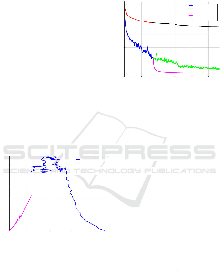
In Figure 6, the convergence of the loss along a

magnitude approximately proportional to MFLOPS is

depicted. The blue curve shows the ﬁrst phase of us-

ing Adam and the green curve shows its continuation

(corresponding to using Adam in a typical way). The

second phase loss of CG (magenta curve) decreases

0 1e+06 2e+06 3e+06 4e+06 5e+06

0.02

0.04

0.06

0.08

0.1

Epochs X M Params X Training Set Length

Loss

Adam Ph.1

CG Ph.1

Adam Ph.2 (<= Adam Ph.1)

CG Ph.2 (<= Adam Ph.1)

CG Ph.2 (<= CG Ph.1)

Figure 6: Empirical loss function development with alter-

native algorithm sequences on the dataset CIFAR-10 and a

ViT architecture. The most effective strategy is the two-

phase training with Adam (blue) and CG (magenta). For

comparison, the green line shows continuation of the Adam

phase, while the red and black lines show the training purely

done with CG.

considerably faster than its Adam counterpart (green

curve). The traditional Adam optimization over all

700 epochs (the blue curve and its continuation by the

green curve) is visibly inferior to the convergence of

the two-phase algorithm (blue and magenta curve).

The advantage of the two-phase algorithm re-

mains substantial, even considering additional for-

ward passes per epoch spent by line search of CG.

For comparison, using CG in both phases, the loss is

depicted by the red and black curves.

This pattern occurred for all investigated model

variants and datasets (ViT variants and VGG5 with

CIFAR-10, CIFAR-100, and MNIST). The sustained

simplicity of this pattern was striking and somewhat

unexpected. There were no indicators for saddle

points or spurious minima, which would become ap-

parent as regions of a very small gradient norm. Once

the gradient norm peak passed, the second-order op-

timization path became straightforward. The ﬁnal re-

sults comparing a pure Adam training run and a two-

phase Adam+CG are presented in Table 1.

Furthermore, in terms of performance metrics

loss and accuracy, the overdetermination ratio of

each benchmark candidate has been evaluated (Hrycej

et al., 2023):

Q =

(7)

with K being the number of training examples, M be-

ing the length of the output vector (usually equal to

the number of classes) and P being the number of

trainable model parameters.

This formula justiﬁes itself by ensuring that the

A Convexity-Dependent Two-Phase Training Algorithm for Deep Neural Networks

Table 1: Final results (loss and accuracy for the training and validation split) from the experiments on the three datasets

MNIST, CIFAR-10, and CIFAR-100 for different variants of ViT and VGG5. The algorithm column indicates the conventional

training with Adam or the proposed second-phase training Adam+CG using the conjugate gradient optimization method.

Model variant Algorithm Train loss Train acc. Val. loss Val. acc. Q

MNIST

vit-mlp Adam 0.0008 0.995 0.0061 0.965 3.9

vit-mlp Adam+CG 0.0001 1.000 0.0044 0.974 3.9

vit-nomlp Adam 0.0003 0.998 0.0064 0.963 11.0

vit-nomlp Adam+CG 0.0002 0.999 0.0053 0.969 11.0

vit-nomlp-wkewq Adam 0.0004 0.998 0.0057 0.967 14.1

vit-nomlp-wkewq Adam+CG 0.0002 0.999 0.0048 0.971 14.1

vit-nomlp-wkewq-wvwo1 Adam 0.0016 0.990 0.0073 0.955 33.5

vit-nomlp-wkewq-wvwo1 Adam+CG 0.0006 0.996 0.0063 0.962 33.5

vgg5-max-relu Adam 0.0001 1.000 0.0014 0.993 4.9

vgg5-max-relu Adam+CG 0.0001 1.000 0.0011 0.994 4.9

CIFAR-10

vit-mlp Adam 0.0091 0.943 0.0997 0.428 3.1

vit-mlp Adam+CG 0.0041 0.970 0.0991 0.435 3.1

vit-nomlp Adam 0.0290 0.819 0.0981 0.428 7.9

vit-nomlp Adam+CG 0.0175 0.891 0.0982 0.444 7.9

vit-nomlp-wkewq Adam 0.0386 0.744 0.0889 0.441 9.9

vit-nomlp-wkewq Adam+CG 0.0270 0.833 0.0881 0.461 9.9

vit-nomlp-wkewq-wvwo1 Adam 0.0567 0.575 0.0775 0.414 19.1

vit-nomlp-wkewq-wvwo1 Adam+CG 0.0527 0.612 0.0738 0.436 19.1

vgg5-max-relu Adam 0.0059 0.967 0.0531 0.710 4.1

vgg5-max-relu Adam+CG 0.0047 0.969 0.0491 0.719 4.1

CIFAR-100

vit-mlp Adam 0.0041 0.706 0.0128 0.155 29.7

vit-mlp Adam+CG 0.0028 0.758 0.0134 0.151 29.7

vit-nomlp Adam 0.0062 0.478 0.0112 0.166 72.6

vit-nomlp Adam+CG 0.0053 0.534 0.0116 0.165 72.6

vit-nomlp-wkewq Adam 0.0069 0.425 0.0108 0.174 88.4

vit-nomlp-wkewq Adam+CG 0.0059 0.487 0.0109 0.176 88.4

vit-nomlp-wkewq-wvwo1 Adam 0.0082 0.291 0.0099 0.157 156.4

vit-nomlp-wkewq-wvwo1 Adam+CG 0.0078 0.326 0.0097 0.164 156.4

vgg5-max-relu Adam 0.0032 0.755 0.0108 0.300 38.9

vgg5-max-relu Adam+CG 0.0032 0.737 0.0102 0.321 38.9

numerator KM is equal to the number of constraints to

be satisﬁed (the reference values for all training exam-

ples). This product must be larger than the number of

trainable parameters for the system to be sufﬁciently

determined. Otherwise, there are inﬁnite solutions,

most of which do not generalize. This is equivalent to

the requirement for the overdetermination ratio Q to

be larger than unity. On the other hand, too large Q

values may explain a poor attainable performance —

the model does not have enough parameters to repre-

sent the input/output relationship. This is the case for

CIFAR-100.

For the evaluation of the hypothesis formulated

in Section 3, only the loss values (that is, MSE) on

the training set are signiﬁcant since this magnitude

is what is directly minimized and thus tests the ef-

ﬁciency of the minimization algorithm. There, sus-

tained superiority of the two-phase concept can be ob-

served.

Nevertheless, the superiority can also be extended

to the accuracies and the validation set measures. The

extent of the generalization gap (the performance dif-

ference between the training and the validation sets)

varies greatly. In most cases, they can be explained by

the overdetermination ratio: its large values coincide

with a small training gap. This does not apply across

model groups; VGG5 generalizes better than ViT for

given model architectures.

Most models used here do not reach peak perfor-

mances reached by optimally tuned models for image

classiﬁcation. They are typically substantially smaller

to allow for the experiment series with a sufﬁcient

number of epochs. Low epoch numbers would bring

about the risk of staying in the initial non-convex re-

KDIR 2025 - 17th International Conference on Knowledge Discovery and Information Retrieval

gion without approaching the genuine minimum.

6 CONCLUSION

Our empirical results strongly support the hypothe-

sis that loss functions exhibit a predictable convexity

structure proceeding from the initial non-convexity

towards ﬁnal convexity, enabling targeted optimiza-

tion strategies that outperform conventional methods.

Initial weight parameters (small random values) fall

into the non-convex region, while a broad environ-

ment of loss minimum is convex. The validity of

this hypothesis can be observed in the development of

the gradient norm in dependence on the instantaneous

loss: a norm growing with decreasing loss indicates

non-convexity, while a shrinking norm suggests con-

vexity.

This can be exploited to identify the swap point

(gradient norm peak) between both. Then, an efﬁcient

non-convex algorithm such as Adam can be applied

in the initial non-convex phase, and a fast second-

order algorithm such as CG with guaranteed super-

linear convergence can be used in the second phase.

A set of benchmarks has been used to test the va-

lidity of the hypothesis and the subsequent efﬁciency

of this optimization scheme. Although they are rel-

atively small to remain feasible with given comput-

ing resources, they cover relevant variants of the ViT

architecture that can be expected to impact convex-

ity properties: using or not using an MLP, deﬁning

the similarity in the attention mechanism symmetri-

cally or asymmetrically, and putting the value vec-

tors of embeddings in a compressed or uncompressed

form (matrices W

and W

). A completely different ar-

chitecture, the convolutional network VGG5, has also

been tested.

The results have been surprisingly unambiguous.

All variants exhibited the same pattern of the gradient

norm increasing towards a swap point and decreasing

after it. The ﬁnal losses with a two-phase algorithm

have always been better than those with a single algo-

rithm (Adam). CG alone did not perform well in the

initial non-convex phase, which caused a considerable

lag so that the convex region was not attained. The

same is true with a single exception for CIFAR-100.

An analogical behavior can be observed for the per-

formance of the validation set, which has been admit-

tedly relatively poor for CIFAR-100 because of the

excessive overdetermination with given models — the

parameter sets seem to have been insufﬁcient for im-

age classiﬁcation with 100 classes. The top-5 accu-

racy on this dataset was more acceptable, over 50 %.

Of course, it must be questioned how far this em-

pirical ﬁnding can be generalized to arbitrary archi-

tectures, mainly to large models. One of the very dif-

ﬁcult questions is the convexity structure of loss func-

tions with arbitrary models or even with a model class

relevant to practice. However, it is essential to note

that there is no particular risk when using the two-

phase method. Gradient norms can be automatically

monitored and deviations from the hypothesis can be

identiﬁed. If there is evidence against a single gra-

dient norm peak corresponding to the swap point, a

non-convex method can be used to continue as a safe

resort. If the hypothesis can be conﬁrmed, there is an

almost certain reward in convergence speed and accu-

racy.

Nevertheless, the next goal of our work is to verify

the hypothesis on a large text-based model.

REFERENCES

Bermeitinger, B., Hrycej, T., Pavone, M., Kath, J., and

Handschuh, S. (2024). Reducing the Transformer Ar-

chitecture to a Minimum. In Proceedings of the 16th

International Joint Conference on Knowledge Discov-

ery, Knowledge Engineering and Knowledge Manage-

ment, pages 234–241, Porto, Portugal. SCITEPRESS.

Chen, C., Shen, L., Zou, F., and Liu, W. (2022). Towards

practical Adam: Non-convexity, convergence theory,

and mini-batch acceleration. J. Mach. Learn. Res.,

23(1):229:10411–229:10457.

Dosovitskiy, A., Beyer, L., Kolesnikov, A., Weissenborn,

D., Zhai, X., Unterthiner, T., Dehghani, M., Min-

derer, M., Heigold, G., Gelly, S., Uszkoreit, J., and

Houlsby, N. (2021). An image is worth 16x16 words:

Transformers for image recognition at scale. In In-

ternational Conference on Learning Representations,

page 21, Vienna, Austria.

Ergen, T. and Pilanci, M. (2023). The Convex Landscape of

Neural Networks: Characterizing Global Optima and

Stationary Points via Lasso Models.

Fletcher, R. and Reeves, C. M. (1964). Function minimiza-

tion by conjugate gradients. The Computer Journal,

7(2):149–154.

Fotopoulos, G. B., Popovich, P., and Papadopoulos, N. H.

(2024). Review Non-convex Optimization Method for

Machine Learning.

Hrycej, T., Bermeitinger, B., Cetto, M., and Handschuh,

S. (2023). Mathematical Foundations of Data Sci-

ence. Texts in Computer Science. Springer Interna-

tional Publishing, Cham.

Keskar, N. S., Mudigere, D., Nocedal, J., Smelyanskiy, M.,

and Tang, P. T. P. (2017). On Large-Batch Training for

Deep Learning: Generalization Gap and Sharp Min-

ima.

Kingma, D. P. and Ba, J. (2015). Adam: A Method for

Stochastic Optimization. 3rd International Confer-

ence on Learning Representations.

A Convexity-Dependent Two-Phase Training Algorithm for Deep Neural Networks

Kirkpatrick, S., Gelatt, C. D., and Vecchi, M. P. (1983).

Optimization by Simulated Annealing. Science,

220(4598):671–680.

Krizhevsky, A. (2009). Learning Multiple Layers of Fea-

tures from Tiny Images. Dataset, University of

Toronto.

LeCun, Y., Bottou, L., Bengio, Y., and Haffner, P. (1998).

Gradient-based learning applied to document recogni-

tion. Proceedings of the IEEE, 86(11):2278–2324.

Levenberg, K. (1944). A method for the solution of cer-

tain non-linear problems in least squares. Quarterly

of Applied Mathematics, 2(2):164–168.

Li, M., Zhang, T., Chen, Y., and Smola, A. J. (2014). Efﬁ-

cient mini-batch training for stochastic optimization.

In Proceedings of the 20th ACM SIGKDD Interna-

tional Conference on Knowledge Discovery and Data

Mining, Kdd ’14, pages 661–670, New York, NY,

USA. Association for Computing Machinery.

Metropolis, N., Rosenbluth, A. W., Rosenbluth, M. N.,

Teller, A. H., and Teller, E. (1953). Equation of State

Calculations by Fast Computing Machines. The Jour-

nal of Chemical Physics, 21(6):1087–1092.

Mockus, J., Eddy, W., and Reklaitis, G. (1997). Bayesian

Heuristic Approach to Discrete and Global Optimiza-

tion: Algorithms, Visualization, Software, and Appli-

cations. Nonconvex Optimization and Its Applica-

tions. Springer US.

Polak, E. and Ribi

ere, G. (1969). Note sur la convergence de

ethodes de directions conjugu

ees. Revue franc¸aise

d’informatique et de recherche op

erationnelle. S

erie

rouge, 3(16):35–43.

Press, W. H., Teukolsky, S. A., Vetterling, W. T., and Flan-

nery, B. P. (1992). Numerical Recipes in C (2nd Ed.):

The Art of Scientiﬁc Computing. Cambridge Univer-

sity Press, USA.

Rinnooy Kan, A. H. G. and Timmer, G. T. (1987). Stochas-

tic global optimization methods part II: Multi level

methods. Mathematical Programming, 39(1):57–78.

Simonyan, K. and Zisserman, A. (2015). Very Deep Con-

volutional Networks for Large-Scale Image Recogni-

tion. ICLR.

KDIR 2025 - 17th International Conference on Knowledge Discovery and Information Retrieval