A Long Short-Term Memory (LSTM) Neural Architecture for Presaging

Stock Prices

Tej Nileshkumar Doshi, Shubham Ghadge, Yamini Gonuguntla, Namirah Imtieaz Shaik,

Ashutosh Mathore and Bonaventure Chidube Molokwu

Department of Computer Science, College of Engineering and Computer Science, California State University,

Sacramento, U.S.A.

Keywords:

Stock Prediction, LSTM, Deep Learning, Financial Time Series, Machine Learning, Forecasting, Time Series

Analysis.

Abstract:

Stock price prediction is crucial for informed investment decisions(Bathla, 2020; Hochreiter and Schmidhuber,

1997). This study explores the application of Long Short-Term Memory (LSTM) architecture for analyzing

and predicting stock prices of major technology companies: Alphabet Inc. (GOOG), Apple Inc. (AAPL),

NVIDIA Corporation (NVDA), Meta Platforms, Inc. (META), and Tesla Inc. (TSLA). The fundamental chal-

lenge addressed is capturing temporal dependencies and complex patterns in ﬁnancial time series data, which

traditional statistical methods often fail to model accurately(Box et al., 1978; Hyndman and Athanasopoulos,

2013). Our methodology involved collecting historical stock data from Yahoo Finance API(Edwards et al.,

2018), preprocessing through normalization and sequence creation(Hochreiter and Schmidhuber, 1997), and

training separate LSTM models for each stock. Results indicate that LSTM models provide satisfactory ac-

curacy with R² scores exceeding 0.93 for most stocks(Li et al., 2023; Selvin et al., 2017), capturing both

short-term and long-term patterns(Panchal et al., 2024; Ouf et al., 2024). The implications are signiﬁcant

for investors and ﬁnancial analysts seeking enhanced predictive tools for market forecasting(Pramod and Pm,

2020).

1 INTRODUCTION

The stock market represents one of the most dy-

namic and complex ﬁnancial systems, characterized

by rapid and unpredictable price movements inﬂu-

enced by macroeconomic indicators, market senti-

ment, geopolitical events, and social media trends

(Edwards et al., 2018; Li et al., 2023; Ouf et al.,

2024). Traditional statistical models like ARIMA and

GARCH, while theoretically sound, often assume sta-

tionarity and linearity, limiting their effectiveness in

capturing the non-linear, volatile nature of real-world

stock data (Box et al., 1978; Hyndman and Athana-

sopoulos, 2013).

The emergence of Machine Learning and Deep

Learning has enabled more sophisticated forecasting

algorithms capable of capturing hidden patterns in se-

quential data. Long Short-Term Memory (LSTM)

networks, a specialized form of Recurrent Neural

Networks, have demonstrated outstanding perfor-

https://orcid.org/0000-0003-4370-705X

mance in modeling temporal sequences by overcom-

ing the vanishing gradient problem through their gat-

ing mechanisms (Hochreiter and Schmidhuber, 1997;

Selvin et al., 2017; Panchal et al., 2024).

This research develops and evaluates an LSTM-

based model for stock price prediction using histori-

cal data from ﬁve major technology companies, com-

paring performance against traditional and alternative

deep learning approaches using metrics like RMSE,

MAE, and R

Score (Bathla, 2020; Li et al., 2023;

Xiao et al., 2024).

2 LITERATURE REVIEW

Recent studies consistently demonstrate LSTM’s su-

periority over traditional approaches for stock pre-

diction (Panchal et al., 2024; Bathla, 2020; Selvin

et al., 2017). (Panchal et al., 2024) showed LSTM

models achieving lower RMSE values compared to

ARIMA across Apple, Google, and Tesla datasets,

Doshi, T. N., Ghadge, S., Gonuguntla, Y., Shaik, N. I., Mathore, A. and Molokwu, B. C.

A Long Short-Term Memory (LSTM) Neural Architecture for Presaging Stock Prices.

DOI: 10.5220/0013691900003985

Paper published under CC license (CC BY-NC-ND 4.0)

In Proceedings of the 21st International Conference on Web Information Systems and Technologies (WEBIST 2025), pages 473-480

ISBN: 978-989-758-772-6; ISSN: 2184-3252

473

while ARIMA failed to capture non-linear dependen-

cies. (Xiao et al., 2024) compared LSTM, GRU,

and Transformer networks on Tesla stock prediction,

concluding LSTM offered the best trade-off between

complexity and accuracy.

(Li et al., 2023) applied LSTM models to tech-

nology stocks including Apple and Nvidia, demon-

strating high accuracy over decade-long price histo-

ries and emphasizing LSTM’s robustness in captur-

ing long-term temporal dependencies. (Ouf et al.,

2024) incorporated Twitter sentiment features into

LSTM models, reporting improved accuracy com-

pared to price-only models. These ﬁndings, supported

by (Selvin et al., 2017; Bathla, 2020; Pramod and Pm,

2020), provide strong motivation for applying LSTM

networks to a broader dataset of ﬁve major technology

stocks.

3 MATERIALS AND

METHODOLOGY

3.1 Data Collection and Preprocessing

Historical stock price data for AAPL, GOOG, META,

NVDA, and TSLA was collected using the Yahoo Fi-

nance API(Edwards et al., 2018; de Prado, 2018),

covering the period from January 1, 2012, to Decem-

ber 21, 2022. The size of the dataset is represented as

a tuple (13805, 7) where 13, 805 indicates the number

of rows and 7 indicates the number of columns. Each

company has 2761 rows of data. The data includes

features like Open, High, Low, Close, and Volume

ﬁelds(Edwards et al., 2018).

3.2 Feature Engineering and Data

Transformation

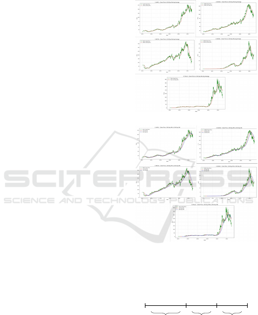
100-Day Moving Average (MA100) and 200-Day

Moving Average (MA200) were computed to provide

additional trend information beyond daily volatility.

These technical indicators help smooth short-term

ﬂuctuations and highlight longer-term trends, with

MA100 capturing medium-term patterns and MA200

focusing on long-term market sentiment(Box et al.,

1978; Hyndman and Athanasopoulos, 2013).

Rather than feeding raw prices directly into the

model, a sliding window approach was applied to cre-

ate sequences. For each stock, sequences of the past

60 days of ’Close’ prices were prepared to predict

the 61st day’s ’Close’ price. A sliding window ap-

proach was adopted to generate the input-output pairs

required by the LSTM model.

Figure 1: 100-Day MA vs Close Price.

Figure 2: 200-Day MA vs 100-Day MA vs Close Price.

We decided to split the data for our model as fol-

lows:

• 80% for Training

• 10% for Validation (from within training set)

• 20% for Testing

2012 2017 2020 2022

Training set Validation set Testing set

Figure 3: Chronological data split into training, validation,

and testing sets.

Fig. 3. above indicates the data split into three

sets. Chronological order was preserved to main-

WEBIST 2025 - 21st International Conference on Web Information Systems and Technologies

474

tain the time-dependent structure of the stock price

data. After sequence generation, the training, val-

idation, and testing sets were reshaped into a 3D

structure required by LSTM layers: (shape) = (sam-

ples,timesteps,features)

Where:

• samples = number of sequences,

• timesteps = 60 (days of history),

• features = 1 (’Close’ price only).

Standard dense layers expect 2D input, but

LSTMs require 3D to maintain temporal relationships

across timesteps.

3.3 Working of LSTM Networks

Long Short-Term Memory (LSTM) networks are an

extension of Recurrent Neural Networks (RNNs),

speciﬁcally designed to overcome the vanishing gra-

dient problem and capture long-range dependencies

in sequential data.

Each LSTM unit is composed of three primary

gates:

• Forget Gate: Decides what information from the

previous cell state should be discarded.

• Input Gate: Determines which new information

should be added to the cell state.

• Output Gate: Controls the information that will

be outputted from the current cell.

At each time step, the LSTM cell takes the current

input and the hidden state from the previous time step,

processes them through the three gates, updates the

internal cell state, and produces a new hidden state.

Mathematically, the gates are computed as fol-

lows:

= σ(W

· [h

t−1

, x

] + b

) (1)

= σ(W

· [h

t−1

, x

] + b

) (2)

= tanh(W

· [h

t−1

, x

] + b

) (3)

= f

∗C

t−1

+ i

∗

(4)

= σ(W

· [h

t−1

, x

] + b

) (5)

= o

∗ tanh(C

) (6)

where:

• σ denotes the sigmoid activation function,

• tanh denotes the hyperbolic tangent activation

function,

• W and b represent the weight matrices and bias

vectors, respectively,

• h

t−1

is the hidden state from the previous time

step,

Figure 4: LSTM Architecture(Molokwu and Kobti, 2019).

• x

is the input at the current time step t.

These mechanisms enable LSTMs to selectively

remember or forget information over long sequences,

making them ideal for modeling time series data such

as stock prices.

Fig. 4. illustrates the internal structure of an

LSTM (Long Short-Term Memory) cell. The LSTM

unit is composed of four primary components: the

Forget Gate, the Input Gate, the Cell State Update,

and the Output Gate.

• The Forget Gate determines which parts of the

previous cell state (C

t−1

) should be discarded

based on the previous hidden state (h

t−1

) and the

current input (x

• The Input Gate decides which new information

should be written into the cell state, again using

the current input and the previous hidden state.

• The Cell State Update combines the output of the

forget and input gates to update the internal cell

memory (C

• The Output Gate generates the new hidden state

) based on the updated cell state and regulates

what information will be passed to the next time

step.

The inputs to the LSTM cell are the previous hid-

den state h

t−1

, the previous cell state C

t−1

, and the

current input x

. The outputs are the updated cell state

and the new hidden state h

. This structure enables

the LSTM to effectively capture both long-term and

short-term dependencies in sequential data.

3.4 Model Architecture

The LSTM model was designed with a Sequential ar-

chitecture:

• LSTM Layer 1: 128 units, return sequences, Input

Shape: (60 timesteps, 1 feature). The ﬁrst LSTM

layer processes each 60-day sequence and learns

intricate temporal dependencies across multiple

trading days. Setting return sequences=True en-

sures that the output of this layer is a full se-

quence (not a single value), which is passed to

A Long Short-Term Memory (LSTM) Neural Architecture for Presaging Stock Prices

475

the next LSTM layer for deeper pattern extraction.

This layer acts as a feature extractor for sequential

data, capturing both short-term and medium-term

trends.

• Dropout Layer 1: 0.3. A Dropout layer is inserted

after the ﬁrst LSTM to randomly deactivate 30%

of the neurons during each training batch. This

technique prevents the model from overﬁtting by

ensuring it does not become too dependent on spe-

ciﬁc neurons. Dropout regularization encourages

generalization over training data.

• LSTM Layer 2: 64 units, no return sequences.

The second LSTM layer receives the sequence

output from the ﬁrst LSTM but collapses it

into a single vector output by setting return se-

quences=False. This vector summarizes the tem-

poral features extracted from the entire 60-day in-

put window. This layer acts as a temporal summa-

rizer, enabling the model to output a single future

price prediction.

• Dropout Layer 2: 0.3. Another Dropout layer is

added to reduce overﬁtting risks even after feature

summarization, ensuring robustness in the learned

representations.

• Dense Output Layer: 1 neuron/unit. The ﬁnal

layer is a Dense (Fully Connected) layer with one

output neuron. It maps the processed sequential

features into a single scalar value — the predicted

closing stock price for the next day.No activation

function is applied because stock price prediction

is a regression task.

3.5 Model Compilation, Training, and

Prediction

After deﬁning the LSTM model architecture, the

model was compiled using:

• Optimizer: Adam The Adam optimizer was cho-

sen due to its adaptive learning rate capabilities,

fast convergence properties, and widespread suc-

cess in deep learning tasks. Adam combines the

advantages of both RMSProp and SGD optimiz-

ers, making it well-suited for noisy and sparse

datasets like ﬁnancial time series.

• Loss Function: Mean Squared Error (MSE) MSE

is the standard loss function for regression tasks

where the goal is to predict continuous values,

such as stock closing prices. It penalizes larger er-

rors more heavily, encouraging the model to pro-

duce highly accurate predictions.

The model compilation stage ensures that the appro-

priate optimization and evaluation settings are pre-

pared before training begins.

Next, the training was performed using the train-

ing set, with validation on a separate validation set to

monitor the model’s generalization ability and detect

any signs of overﬁtting.

• Number of Epochs: 100

• Batch Size: 32 samples per training step

During training, the model learned to minimize the

MSE loss on the training data while maintaining sta-

ble validation loss to ensure good generalization to

unseen data.

The training process produced a history object

containing loss and validation loss values for each

epoch, which were later used for plotting learning

curves.

Finally, after the model completed training, pre-

dictions were generated on:

• Training set (for internal performance assess-

ment),

• Validation set (to monitor overﬁtting),

• Testing set (to evaluate real-world generalization).

Since the model was trained on normalized (scaled)

data between [0,1], the predicted outputs needed to be

inverse transformed back to their original price scale

for meaningful interpretation. Inverse transformation

was performed using the previously ﬁtted MinMaxS-

caler on both:

• Predicted values (train, validation, test sets),

• True target values (ground truth for train, valida-

tion, test sets).

This rescaling ensures that evaluation metrics like

RMSE, MAE, and R² Score, and graphical visualiza-

tions (actual vs predicted prices) are reported in real

stock price units (e.g., 150,300).

3.6 Frameworks, Programming

Languages, and Libraries

The proposed LSTM-based stock price prediction

system was implemented using the following soft-

ware tools and libraries:

• Programming Language: Python 3.8+

• Deep Learning Framework: TensorFlow 2.x

(with Keras API)

• Machine Learning Utilities: scikit-learn

• Financial Data Access: yﬁnance

• Data Manipulation: pandas and NumPy

• Visualization: matplotlib

WEBIST 2025 - 21st International Conference on Web Information Systems and Technologies

476

4 EXPERIMENT AND RESULTS

This section presents the outcomes of training the

LSTM models, analyzing the learning behavior, eval-

uating the predictive performance using standard met-

rics.

4.1 Evaluation Metrics

Model performance was assessed using four standard

regression metrics:

• Mean Squared Error (MSE): Measures the aver-

age squared difference between actual and pre-

dicted values.

• Root Mean Squared Error (RMSE)(Kumar et al.,

2021): Square root of MSE, interpretable in the

same units as stock price.

• Mean Absolute Error (MAE): Average of absolute

differences between actual and predicted values.

• Coefﬁcient of Determination (R² Score): Mea-

sures how well predictions approximate real data

(1 = perfect prediction).

The Table 1 below shows the evaluation metrics for

each of the companies.

Table 1: Model Performance Metrics for Different Compa-

nies.

Company MSE RMSE MAE R

Score

Apple 11.73 3.42 2.68 0.9576

Google 25.32 5.03 4.33 0.9314

Meta 78.86 8.88 6.61 0.9877

Nvidia 6.43 2.54 2.19 0.7741

Tesla 204.77 14.31 10.61 0.9367

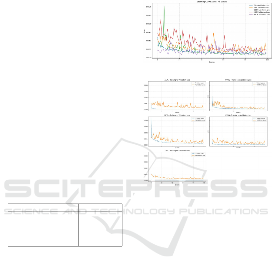
4.2 Learning Curves

Fig. 5. presents the validation loss across all ﬁve com-

panies over 100 training epochs. The validation loss

serves as an indicator of the model’s ability to gener-

alize to unseen data. Stocks like Google and Apple

showed consistent and low validation losses, suggest-

ing stable and effective training. On the other hand,

Meta and Tesla experienced more ﬂuctuation in vali-

dation loss, particularly during early epochs. This in-

stability reﬂects the inherent volatility of these stocks

in the given timeframe, making prediction more chal-

lenging. Nevertheless, all models showed conver-

gence trends, and none displayed sustained overﬁtting

behavior.

Figure 5: Learning Curves for 5 Companies.

Figure 6: Training Loss vs Validation Loss.

4.3 Training and Validation Loss

Analysis

To better understand the learning behavior of the

LSTM model, both Training Loss and Validation Loss

were recorded during training for each stock. The

curves are presented in the Fig. 6. for the ﬁve compa-

nies individually.

The analysis of the curves revealed the following

observations:

• For most stocks (Apple, Google, Meta), the train-

ing and validation losses decreased steadily and

remained close to each other, indicating that the

model generalized well without signiﬁcant over-

ﬁtting.

• Nvidia exhibited slightly slower convergence ini-

tially, but validation loss ultimately stabilized af-

ter around 50 epochs.

• Tesla’s stock showed higher validation loss ﬂuc-

tuations during early epochs, which can be at-

tributed to Tesla’s high volatility in the real

stock market during the studied period (especially

2020-2022).

A Long Short-Term Memory (LSTM) Neural Architecture for Presaging Stock Prices

477

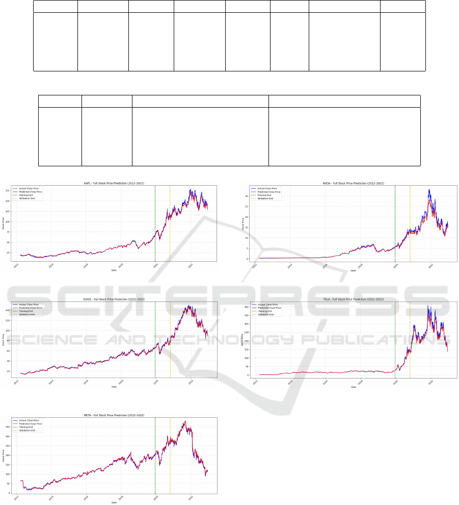
Table 2: RMSE Comparison of Our LSTM Model with Other Approaches from Literature.

Company Our LSTM [1] LSTM [1] ARIMA [2] LSTM [2] GRU [2] Transformer [3] LSTM

Apple 3.42 5.52 13.60 N/A N/A N/A 18.89

Google 5.03 4.66 7.15 N/A N/A N/A 18.89

Meta 8.88 N/A N/A N/A N/A N/A N/A

Nvidia 2.54 N/A N/A N/A N/A N/A N/A

Tesla 14.31 12.38 23.98 26.09 18.44 16.40 N/A

Table 3: Comparison of R

Scores Between Our LSTM Model and Results from (Ouf et al., 2024).

CompanyOur LSTM[4] LSTM (Sentiment Analysis) [4] LSTM (No Sentiment Analysis)

Apple 95.76% 91% 98%

Google 93.14% 88% 95%

Meta 98.77% N/A N/A

Nvidia 77.41% N/A N/A

Tesla 93.67% 73% 55%

Figure 7: LSTM model prediction graph of Apple.

Figure 8: LSTM model prediction graph of Google.

Figure 9: LSTM model prediction graph of Meta.

4.4 Full Time Predictions

The full timeline plots comparing actual and predicted

closing prices for each stock across the training, val-

idation, and testing periods revealed several key in-

sights:

• We see in Fig. 7. Fig. 8. Fig. 9. for

Figure 10: LSTM model prediction graph of Nvidia.

Figure 11: LSTM model prediction graph of Tesla.

Apple, Google, and Meta stocks respectively,

demonstrated excellent alignment between actual

and predicted prices across the entire 2012–2022

timeline, with minimal deviation during both sta-

ble and volatile periods.

• In Fig. 10. Nvidia’s stock showed good general

predictive performance but had slight underﬁt-

ting during rapid market changes, suggesting that

additional features (such as market news senti-

ment) could further enhance the model for highly

volatile stocks.

• Tesla’s stock in Fig. 11, due to its extremely high

volatility in 2020–2022 (e.g., stock splits, market

sentiment shifts), exhibited larger prediction er-

rors during sudden spikes. However, the LSTM

model was still able to capture the overall upward

trend and major turning points reasonably well.

WEBIST 2025 - 21st International Conference on Web Information Systems and Technologies

478

4.5 Comparative Result Analysis

To benchmark our proposed LSTM model, we com-

pared our experimental results in Table 2 and Table 3

against four other published IEEE papers:

In all cases, the LSTM model successfully learned

the temporal dependencies in the stock price se-

quences and was able to generalize well to unseen

testing data.

Importantly, no signiﬁcant divergence was ob-

served between actual and predicted prices toward the

end of the testing period for any of the stocks, con-

ﬁrming the model’s stability and robustness.

Furthermore, the prediction plots clearly illus-

trated that the LSTM model was not merely mem-

orizing training data but was genuinely learning un-

derlying patterns and trends that could be generalized

across time periods.

5 DISCUSSION AND

LIMITATIONS

The experimental results demonstrate LSTM’s high

effectiveness for stock price forecasting, with R²

scores exceeding 0.9 for most stocks conﬁrming

successful capture of complex temporal dependen-

cies. Comparative analysis showed LSTM consis-

tently outperforming ARIMA and matching or ex-

ceeding GRU and Transformer performance. Key

limitations include: (1) univariate analysis using only

closing prices, missing beneﬁts from technical indi-

cators like RSI, MACD, or sentiment analysis; (2)

single-step prediction limiting real-world trading ap-

plicability; (3) computational expense compared to

simpler models; and (4) performance degradation on

highly volatile stocks like Tesla during extreme mar-

ket conditions. Despite limitations, the study con-

ﬁrms LSTM networks as reliable tools for ﬁnancial

time series modeling, with architecture suitable for

algorithmic trading systems, risk modeling, and port-

folio optimization strategies.

6 CONCLUSION AND FUTURE

WORK

This study demonstrates LSTM neural networks’ ef-

fectiveness in predicting stock prices using historical

closing price data. Key ﬁndings include strong gen-

eralization (R² ¿ 0.93 for most stocks), stable training

without overﬁtting, robust performance across volatil-

ity levels, and superior benchmark performance com-

pared to traditional ARIMA and competitive deep

learning models. Results conﬁrm LSTM’s power

in capturing non-linear, time-dependent structures in

stock market data. The model’s modularity allows

easy future extensions and real-world applications in

portfolio management and algorithmic trading. Fu-

ture enhancements could incorporate additional fea-

tures (volume, volatility indicators, sentiment analy-

sis), extend to multi-step predictions, combine with

attention mechanisms, include macroeconomic indi-

cators, deploy real-time systems with continuous re-

training, and apply explainability tools for transparent

decision-making.

ACKNOWLEDGMENT

The authors would like to sincerely thank Dr.

Bonaventure Chidube Molokwu at California State

University, Sacramento, for their invaluable guidance,

support, and constructive feedback throughout the du-

ration of this project. Their encouragement and in-

sightful comments were instrumental in shaping the

methodology, experiments, and analysis presented in

this study.

We also acknowledge the availability of open-

source ﬁnancial data APIs such as Yahoo Finance and

the use of powerful deep learning libraries like Ten-

sorFlow and Scikit-learn, which greatly facilitated the

successful completion of this project.

REFERENCES

Bathla, G. (2020). Stock price prediction using lstm and svr.

In 2020 Sixth International Conference on Parallel,

Distributed and Grid Computing (PDGC), pages 211–

214. IEEE.

Box, G. E. P., Jenkins, G. M., Reinsel, G. C., and Ljung,

G. M. (1978). Time series analysis: Forecasting and

control. The Statistician, 27:265–265.

de Prado, M. M. L. (2018). Advances in ﬁnancial machine

learning: Numerai’s tournament (seminar slides).

Electrical Engineering eJournal.

Edwards, R. D., MaGee, J., and Bassetti, W. H. C. (2018).

Technical analysis of stock trends. CRC Press, Boca

Raton, 11th edition.

Hochreiter, S. and Schmidhuber, J. (1997). Long short-term

memory. Neural Computation, 9(8):1735–1780.

Hyndman, R. J. and Athanasopoulos, G. (2013). Forecast-

ing: principles and practice. OTexts.

Kumar, A., Alsadoon, A., Prasad, P. W. C., Abdullah, S. H.,

Rashid, T. A., Pham, D. T. H., and Nguyen, T. Q. V.

(2021). Generative adversarial network (gan) and en-

hanced root mean square error (ermse): deep learn-

A Long Short-Term Memory (LSTM) Neural Architecture for Presaging Stock Prices

479

ing for stock price movement prediction. Multimedia

Tools and Applications, 81:3995–4013.

Li, Z., Yu, H., Xu, J., Liu, J., and Mo, Y. (2023). Stock mar-

ket analysis and prediction using lstm: A case study

on technology stocks. Innovations in Applied Engi-

neering and Technology.

Molokwu, B. C. and Kobti, Z. (2019). Spatial event pre-

diction via multivariate time series analysis of neigh-

boring social units using deep neural networks. In

2019 International Joint Conference on Neural Net-

works (IJCNN), pages 1–8. IEEE.

Ouf, S., Hawary, M. E., Aboutabl, A., and Adel, S. (2024).

A deep learning-based lstm for stock price prediction

using twitter sentiment analysis. International Jour-

nal of Advanced Computer Science and Applications.

Panchal, S. A., Ferdouse, L., and Sultana, A. (2024). Com-

parative analysis of arima and lstm models for stock

price prediction. In 2024 IEEE/ACIS 27th Interna-

tional Conference on Software Engineering, Artiﬁ-

cial Intelligence, Networking and Parallel/Distributed

Computing (SNPD), pages 240–244. IEEE.

Pramod, B. and Pm, M. S. (2020). Stock price predic-

tion using lstm. Test Engineering and Management,

83(3):5246–5251.

Selvin, S., Vinayakumar, R., Gopalakrishnan, E. A.,

Menon, V. K., and Soman, K. (2017). Stock price

prediction using lstm, rnn and cnn-sliding window

model. In 2017 International Conference on Ad-

vances in Computing, Communications and Informat-

ics (ICACCI), pages 1643–1647. IEEE.

Xiao, J., Deng, T., and Bi, S. (2024). Comparative analysis

of lstm, gru, and transformer models for stock price

prediction. In Proceedings of the International Con-

ference on Digital Economy, Blockchain and Artiﬁcial

Intelligence.

WEBIST 2025 - 21st International Conference on Web Information Systems and Technologies

480