Machine Learning-Based Approaches to Forecasting Housing Prices

in the Canadian Market

Yuhao Wen

The Faculty of Arts & Science, University of Toronto, 761 Bay Street, Toronto, Canada

Keywords: Machine Learning, Canada Housing Market, House Price Forecasting.

Abstract: Housing prices are one of the key indicators for measuring the state of the real estate market. Establishing an

efficient housing price forecasting model is of considerable importance to consumers, investors, and

policymakers. In the context of Canadian research, scholars have constructed several regression models to

predict housing prices. However, there remains a paucity of systematic research on model comparison and

hybrid models. This study utilizes Canadian housing price data and employs a data preprocessing technique

involving least absolute shrinkage and selection operator (LASSO) feature selection. Multiple regression

models are then constructed including multiple linear regression (MLR), random forest (RF), extreme gradient

boosting (XGBoost), and a hybrid model integrating RF and XGBoost. During the model building process,

GridSearchCV method is applied to perform hyperparameter tuning for the machine learning models RF and

XGBoost. The models are subsequently compared and analyzed using metrics including Mean Absolute Error

(MAE), Root Mean Squared Error (RMSE) and R-squared to identify the most effective model for housing

price prediction within the Canadian context. The study revealed that the hybrid model, comprising a linear

weighted combination of RF and XGBoost, demonstrated the most efficacy in housing price forecasting.

1 INTRODUCTION

In Canada, housing typically constitutes the largest

segment of households' asset portfolios, with its value

approximating the aggregate of a portion of

investments in major financial assets, including

stocks, insurance, and pensions (Relations, 2011).

Research has previously indicated that housing price

fluctuations and mortgage pressure exert a substantial

influence on individuals' well-being. Home buyers

frequently encounter elevated loan pressures during

periods of increasing housing prices, while declining

housing prices may result in negative asset status,

which can subsequently cause health concerns such

as anxiety and depression (Clair, 2016). The

development of a more accurate housing price

prediction model can serve as a crucial indicator of

the real estate market state. Such a model can assist

the government in conducting timely macro policy

adjustments, thereby mitigating the adverse impact on

people's living conditions and even their physical and

mental health.

https://orcid.org/0009-0001-9030-7895

In housing price forecasting studies, the

multivariate linear regression (MLR) model is

typically the primary method of consideration. Zhang

employed the MLR model to forecast housing prices

and utilized the Spearman correlation coefficient to

analyze the primary influencing factors (Zhang,

2021). While the MLR model can effectively predict

housing prices to a certain extent, its predictive ability

is often inferior to more complex machine learning

models because housing prices are influenced by

numerous non-linear factors. In recent years, machine

learning methods have seen increased utilization in

housing price forecasting. Adetunji et al. employed

the random forest (RF) method to predict Boston

housing prices and evaluated the model's

performance on the relevant dataset, with the error

margin between the predicted and actual house prices

being within ±5 (Adetunji, 2022). Avanija et al.

employed extreme gradient boosting (XGBoost) for

housing price forecasting and proposed an enhanced

data preprocessing method, encompassing data

cleaning, anomaly value removal, Z-score

standardization, and One-Hot encoding. The research

348

Wen, Y.

Machine Learning-Based Approaches to Forecasting Housing Prices in the Canadian Market.

DOI: 10.5220/0013689900004670

Paper published under CC license (CC BY-NC-ND 4.0)

In Proceedings of the 2nd International Conference on Data Science and Engineering (ICDSE 2025), pages 348-354

ISBN: 978-989-758-765-8

findings indicate that XGBoost demonstrates efficacy

in housing price prediction (Avanijaa, 2021). Beyond

the examination of individual models, some scholars

have also engaged in a comparative analysis of

multiple models. For instance, Sharma, Harsora, and

Ogunleye examined the application of multiple

machine learning models in housing price prediction,

finding that XGBoost exhibited the most optimal

prediction performance within the context of the

studied data (Sharma, 2024).

Research on housing price forecasting in the U.S.

using machine learning and statistical methods has

been extensive and systematic. However, in Canada,

housing price forecasting studies are comparatively

few, and there is no systematic comparison of models.

This study aims to address the research gap by

assessing and comparing the performance of MLR,

RF, in the Canadian context. The goal is to determine

the optimal prediction model.

The structure of the paper is as follows: the

Methods section describes the data sources and

preprocessing procedures, and outlines the theoretical

foundations of the selected models. Least Absolute

Shrinkage and Selection Operator(LASSO) will be

applied to fix the missing value problem. The Results

and Discussion section systematically compares the

predictive performance of multiple linear regression,

machine learning models, and the hybrid model to get

the best model. Analyzing the causes of the model

results, explaining the advantages and limitations of

the models. Finally, the Conclusion section

synthesizes the key findings and puts forward

recommendations.

2 METHODS

2.1 Data Description

Prior to the formulation models for analysis, it is

imperative to possess a comprehensive understanding

of the dataset. This study utilizes the Canadian

Housing dataset on Kaggle (Bulana, 2025), which

originally contains 44,896 observations of housing

information on multiple Canadian cities. In reality,

housing prices are influenced by a multitude of

factors. This dataset encompasses 23 features,

including the target variable to be studied, as well as

diverse information such as the basic composition of

the property, the structure of the house, the

geographical location, and the decoration. The names

of the interested features and corresponding meanings

are delineated in the table below.

Table 1: Variable name and description.

Features Descri

tion

Cit

The name of the cit

Province

The province or territory

where the property is

locate

Latitude

The latitude coordinate of

the location of the

ropert

Longitude

The longitude coordinate

of the location of the

ropert

Price

The market price of the

roperty in CAD

Bedrooms

The number of bedrooms

in the

ert

Bathrooms

The number of bathrooms

in the propert

Property Type

The category of the

ropert

Square Footage

The total indoor space of

the

ert

in s

uare feet

Garage

Indicates whether the

ert

has a

ara

Parking

Indicates whether the

property has a parking

ace

Fireplace

Indicates whether the

roperty has a fireplace

Heatin

e of heatin

stem

Sewe

e of sewer s

ste

2.2 Data Preprocessing

The primary concern in managing the dataset is the

handling of missing values, which is particularly

critical due to the high proportion of missing data in

four sub-variables. Specifically, Basement has 67%

of its values missing, Exterior has 61% missing,

Flooring has 66% missing, and Roof has the highest

proportion, with 78% of its data absent. Additionally,

certain other variables possess a small number of

missing values. When directly utilizing the mode for

imputation, the true distribution of the data may not

be accurately recovered, potentially leading to

significant deviations and compromising the stability

and predictive capability of the model. To

scientifically determine the retention of these

variables, we employ LASSO feature selection

method to assess their contribution to the target

variable. The LASSO results indicate that, for

variables of low importance, direct deletion of the

variable is preferable to interpolation, as this

approach reduces data noise and enhances the model's

generalizability.

LASSO is a regularized regression method widely

used for feature selection. LASSO uses an L1

Machine Learning-Based Approaches to Forecasting Housing Prices in the Canadian Market

349

regularization term to compress regression

coefficients, effectively screening out irrelevant

variables (Sharma, 2024). Here's the common form of

the objective function of LASSO:

𝑚𝑖𝑛





(

𝑦



−𝛽



−𝑥





𝛽

)



+𝜆

𝛽















(1)

After running the LASSO model, a bar chart of

feature importance is generated. The regression

coefficients of the Basement, Exterior, Flooring,

Acreage and Roof variables approximate 0,

suggesting that they exert minimal influence on the

prediction of the target variable. Consequently, the

deletion of these variables is a reasonable action, as it

reduces data noise and enhances the model's stability.

Following the elimination of the columns

corresponding to the five variables, the rows

containing missing values for the other variables were

also eliminated, resulting in a total of 38,242

observations in the dataset. Notably, the proportion of

'False' outcomes for the categorical variables

Waterfront, Pool, Garden, and Balcony all exceeds

95%. Indicating that they carry a single piece of

information and may have adversely impacted the

performance of certain models, which may also be

discarded. Given the even distribution of the City

variables, simple random sampling (SRS) was

employed to enhance the efficiency of the model

training and to ensure sufficient representativeness

(Noor, 2022). Ultimately, 5,000 samples were

randomly selected to constitute the final dataset. The

dataset was divided into 80% for training and 20% for

testing.

2.3 Model Selection

2.3.1 MLR

The MLR model is a statistical model based on linear

assumptions. It is used to simulate the linear

relationship between the target variable and multiple

features. The mathematical expression for the model

is as follows:

𝑌=𝛽



+𝛽



𝑥



+𝛽



𝑥



+ ··· +𝛽



𝑥



+𝜀 (2)

Where Y is the target variable(house price); 𝛽



is the

intercept term(the house price when all characteristic

values are 0); 𝛽



𝛽



… 𝛽



are the regression

coefficients of the characteristics, showing the degree

of influence of each characteristic on the house price;

𝑥



𝑥



…𝑥



encompass various characteristics of the

house; 𝜀 is the error term. The MLR model is simple

and intuitive, but its performance may be suboptimal

in complex nonlinear relationships. We have

introduced other nonlinear models for comparative

analysis to address this.

2.3.2 Random Forest

Random forest is an ensemble learning method based

on decision trees. It constructs multiple trees to

reduce the risk of overfitting and improve stability.

This model uses bootstrap sampling and features

random selection to construct trees, and performs

final prediction by means of ensemble learning. The

prediction method is as follows:

𝑌



𝑇



𝑓









(

𝑋

)

(3)

Here T denotes the number of decision trees;

𝑓



(𝑋) signifies the prediction result of the tth decision

tree. The final prediction value is the average of all

decision trees. In comparison with linear regression,

random forests employ a combination of multiple

decision trees, thereby enhancing their capacity to

model non-linear relationships and reducing their

sensitivity to noise in individual data points.

Additionally, random forests mitigate variance and

the risk of overfitting by integrating the predictions of

multiple decision trees, typically by averaging (in

regression tasks) or majority voting (in classification

tasks). Finally, random forests randomly select

features for splitting during training, allowing the

model to automatically ignore redundant or irrelevant

features and thus maintain high computational

efficiency in high-dimensional data.

2.3.3 XGBoost

XGBoost is an ensemble learning method based on

gradient boosted decision trees (GBDT). It employs a

weighted learning (boosting) strategy to enhance

prediction capabilities through gradual optimization.

The tth prediction expression for XGBoost is as

follows:

𝑌

()



=𝑌

()



+𝜂

𝑓



(𝑋)

(4)

Where 𝑌

()



denote the predicted value of the

model in the previous t-1 cycle; 𝑓



(𝑋) is the new

decision tree obtained in this round of training; 𝜂 is

the learning rate, defined as the rate at which the new

decision tree is incorporated into the original model.

ICDSE 2025 - The International Conference on Data Science and Engineering

350

XGBoost optimizes the training of models by

minimizing the target loss function, such as mean

squared error (MSE). In comparison with traditional

GBDT, XGBoost incorporates a regularization term

into the loss function, thereby enhancing the model's

generalization ability and mitigating the risk of

overfitting. The mathematical expression for this

process is typically expressed as follows:

𝐿=𝑙

(

𝑦



,𝑦





)

+Ω

(

𝑓



)













(5)

(

𝑓



)

=𝛾𝑇+

𝜆𝑤











(6)

Where 𝑙

(

𝑦



,𝑦





)

is the standard loss function;

(

𝑓



)

is the regularization term; T is the current number of

leaf nodes in the decision tree; 𝛾 is the leaf node

number penalty coefficient; 𝜆 is the coefficient used

to limit the weight of the leaf node; 𝑤





is the weight

of the jth leaf node.

2.3.4 Hybrid Regression (Random forest +

XGBoost)

A hybrid model is generally composed of two or more

base models, which combine the advantages of

different models to enhance prediction performance.

In this study, the Linear Weighted Combination

Method is employed, with Random Forest (RF) and

XGBoost (XGB) selected as the base models. The

weights are adjusted to construct a new combined

model. The mathematical expression of the hybrid

model is as follows:

𝑌





=𝑤



𝑌





+𝑤



𝑌





𝑤



+𝑤



(7)

Where 𝑤



and 𝑤



indicate the weight of RF and

XGBoost in the prediction result, respectively; 𝑌





the predicted value for RF; 𝑌





is the predicted

value for XGBoost.

2.3.5 Model Evaluation

In this study, mean absolute error(MAE) and root

mean squared error(RMSE) will be considered as

indicators of model performance.

𝑀𝐴𝐸=

𝑁



𝑦



−𝑦











(8)

𝑅𝑀𝑆𝐸=



𝑁



(

𝑦



−𝑦





)







(9)

Where N is the total number of samples; 𝑦



is the

ith real value; 𝑦



is the ith predicted value. In

addition, Chicco et al. have noted that R² can better

reflect the quality of a regression model than MAE

and RMSE and can more accurately measure the

variance explained by the dependent variable (Chicco,

2021). Therefore, this study also uses R² as one of the

evaluation indicators, and these three will be used

together to evaluate the performance of the model.

𝑅



=1−

𝑁

∑(

𝑦



−𝑦





)







𝑁

∑(

𝑦



−𝑦





)







(10)

Where 𝑦



 is the mean of real value.

In general, Lower MAE and RMSE indicate better

model performance, while a higher R-squared

signifies greater explanatory power.

3 RESULTS AND DISCUSSION

2.3.1 Basic EDA Results

Before building the model, EDA will be used to

understand the data set and the relationships between

variables. Initially, Figure 1 is plotted to show

histograms for numeric variables. This is used to

assess the distribution of the data, its skewness

characteristics, and the presence of outliers.

Figure 1: Histograms of Numerical Variables. (Picture

credit: Origins)

The results show that most variables have right-

skewed distributions. For the target variable, most

houses in the dataset are low-priced with few high-

priced properties. House size and number of

Machine Learning-Based Approaches to Forecasting Housing Prices in the Canadian Market

351

bedrooms show long-tailed distributions with

potential outliers. Latitude and longitude variables

have dispersed distributions, indicating that property

data originates from multiple geographic areas.

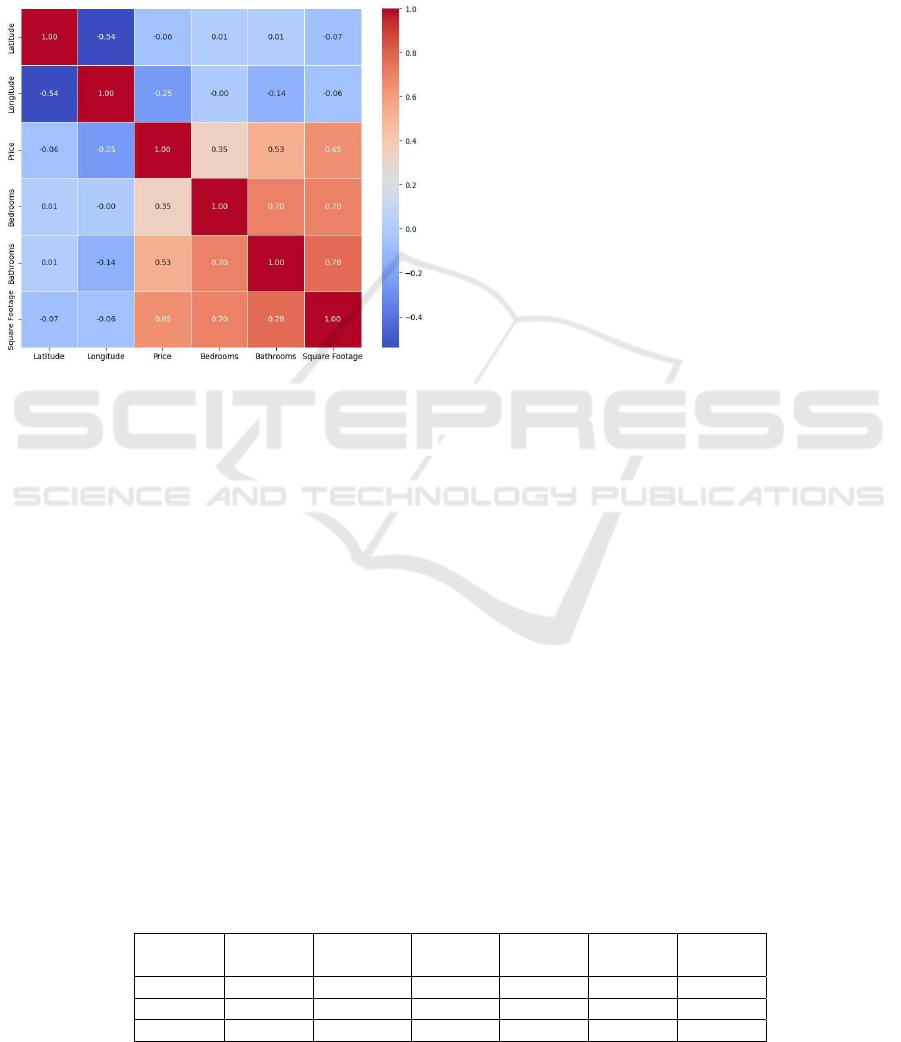
After analysing histograms, Figure 2 is generated

to show heatmap of correlation matrix for numerical

variables. This method uses color shades to represent

correlation levels. It is often used to analyse linear

relationships between variables.

Figure 2: Heatmap of correlation Matrix. (Picture credit:

Original)

In Figure 2, the strength of the positive or negative

correlation is indicated by the intensity of the red or

blue in the figure, respectively. Lighter colors

indicate weaker linear relationships between the

variables. The heatmap indicates a substantial impact

of bathroom dimensions and square footage on the

target variable, exhibiting a robust positive

correlation. This suggests that houses with more

bedrooms and bathrooms tend to command higher

prices, which aligns with prevailing market logic in

the real estate sector. In contrast, the correlation

between the number of bedrooms and house price is

relatively weak, suggesting that while the number of

bedrooms may influence house price, its impact is

less significant than that of house size and the number

of bathrooms. This may be because house size and the

number of bathrooms can more directly reflect the

comfort and market value of the house. It is

noteworthy that the geographical variables exhibit a

low correlation, suggesting that while housing price

is influenced by location, the linear relationship is not

readily apparent. In practice, the impact of location on

housing prices is often non-linear, as evidenced by the

significant variation in housing prices between city

centers and suburbs, which can be challenging to

measure through a simple linear correlation.

3.2 Model results and discussion

Table 2 shows the MAE, RMSE, and R-squared

values for the models MLR, RF, and XGBoost. The

evaluation shows that RF and XGBoost perform

better than MLR. The R-squared value for MLR is

0.5911, and the MAE and RMSE are 592,927.3 and

1,064,716.9. This shows that MLR doesn't effectively

capture the complex patterns in the data. XGBoost

and RF perform better than the others, with R-squared

values of 0.7887 and 0.8007, respectively. XGBoost

has the lowest MAE of 286,103.7, showing its

effectiveness in reducing mean error. RF has the

lowest RMSE of 743,287.8, showing its slightly

better ability to control larger errors.

GridSearchCV is a tool for hyperparameter

optimization that systematically searches for the

optimal hyperparameter combination to improve the

performance of machine learning models. Alemerien

et al. used GridSearchCV to optimize XGBoost and

Random Forest and achieved the best classification

accuracy in the cardiovascular disease prediction task

(Alemerien, 2024). As MLR does not entail

hyperparameter tuning, this method exclusively

focuses on optimizing RF and XGBoost to enhance

the model's predictive capabilities. The optimization

outcomes are depicted in the latter half of Table 2,

including the MAE, RMSE, and R-squared scores.

Prior to the implementation of optimization

techniques, both RF and XGBoost exhibited superior

performance in distinct error metrics. However, after

the optimization process, RF has surpassed XGBoost

in all error metrics, substantiating its enhanced

capacity for generalization. Specifically, the MAE of

RF has decreased from 296,429.0 to 281,715.4,

RMSE has dropped from 743,287.8 to 717,681.5, and

R-squared has improved to 0.8142, indicating further

enhancement in its fitting capabilities. Similarly, the

MAE of XGBoost has declined to 282,458.4, RMSE

has decreased to 763,109.8, and R-squared has

increased to 0.7899. Despite these improvements, the

overall error has remained higher than that of RF.

Table 2: Single Model Result Comparison.

Model

MAE

Before

RMSE

Before

R Square

Before

MAR

Afte

RMSE

Afte

R Square

Afte

MLR 592927.3 1064716.9 0.5911

RF 296429.0 743287.8 0.8007 281715.4 717681.5 0.8142

XGBoost 286103.7 765342.7 0.7887 282458.4 763109.8 0.7899

ICDSE 2025 - The International Conference on Data Science and Engineering

352

In order to enhance the predictive performance of

the model, this study then employs the Weighted

Linear Combination method to construct three hybrid

models that integrate optimized RF and XGBoost

regression. To investigate the impact of distinct

model combinations on the ultimate prediction

outcomes, three distinct weight configurations have

been applied. The weight distribution of the hybrid

model is as follows:

• Hybrid Model 1: 33% RF + 67% XGBoost

• Hybrid Model 2: 50% RF + 50% XGBoost

• Hybrid Model 3: 67% RF + 33% XGBoost

The results of the three models are shown in Table

3, including the MAE, RMSE and R-squared score of

each hybrid model.

Table 3: Performance of Hybrid Models (RF + XGBoost).

Model MAE RMSE R S

uare

33%RF+67%XGBoost 271930.1 716654.9 0.8147

50%RF+50%XGBoost 270540.6 704325.8 0.8211

67%RF+33%XGBoost 271665.6 700515.9 0.8230

The experimental results demonstrate that the

hybrid model exhibits superior performance in

comparison to the individual models. This

phenomenon can be attributed to the ability of the

hybrid model to combine the advantages of multiple

models and mitigate the limitations of a single model.

Specifically, as the RF weight increases, the RMSE

of the hybrid model experiences a gradual decrease,

while the R-squared value undergoes a corresponding

gradual increase. Among three models, Hybrid Model

3 demonstrated the most optimal performance, with

an MAE of 271,665.6, a RMSE reduced to 700,515.9,

and an R-squared increased to 0.8230. These findings

suggest that this model exhibits superiority in terms

of overall error. Hybrid Model 2 also performs well,

with an RMSE of 704,325.8 and an R-squared of

0.8211, which was slightly lower than the optimal

model but still better than the single model. Hybrid

Model 1 has an RMSE of 716,654.9 and an R2 of

0.8147, which is better than XGBoost alone but

slightly inferior to the other two combinations.

Overall, Hybrid Model 3 demonstrates the highest

R-squared among all models, indicating its optimal

overall fitting ability. Notably, its MAE is marginally

higher than that of Hybrid Model 2, reflecting a

potential trade-off in hybrid model construction.

However, when considering RMSE, Hybrid Model 3

exhibits the most effective control over extreme

errors, indicating enhanced stability in its prediction

errors. Based on a comprehensive evaluation of these

indicators, this study recommends Hybrid Model 3 as

the optimal model.

4 CONCLUSIONS

This study comparatively analyzes the predictive

performance of various regression models based on

Canadian housing price data, with the objective of

investigating the advantages of hybrid models in

housing price prediction tasks. The experimental

results demonstrate that hybrid models consisting of

multiple models exhibit superior performance in

terms of all evaluation metrics (MAE, RMSE, R-

squared), indicating that hybrid models can enhance

prediction accuracy more effectively. The superiority

of hybrid models is primarily attributed to their

capacity to integrate the characteristics of different

base models, thereby enhancing each other's

performance. Specifically, XGBoost has been shown

to possess strong generalization ability, while RF has

been demonstrated to perform better in controlling

large errors. By employing a linear weighting

approach, the hybrid model designed in this study

capitalizes on the strengths of both methods, thereby

achieving enhanced overall error control and fitting

ability. Among the three hybrid models constructed,

the model with a weight distribution of 67% RF +

33% XGBoost demonstrated the strongest overall

performance in all metrics, as evidenced by the lowest

RMSE and the highest R-squared. This finding

suggests that this model offers the most optimal

overall performance in the house price prediction

task.

This study fills the gap in the lack of systematic

comparative analysis in the modeling of Canadian

housing price analysis, and makes improvements in

data processing, feature selection, and model

optimization. In data preprocessing, this study uses

the LASSO feature selection method to identify

features that have a small impact on the target

variable, thereby improving data quality when

dealing with missing value issues. In the model

building process, GridSearchCV is used for

hyperparameter optimization to improve the

prediction performance of the regression model. In

addition, a hybrid model is constructed by integrating

multiple regression models to further improve the

overall fit and prediction stability. The practical

Machine Learning-Based Approaches to Forecasting Housing Prices in the Canadian Market

353

experience of this study can provide a valuable

reference for follow-up research.

In subsequent research, in addition to further

optimizing the performance of individual models, the

focus may shift to the exploration of combination

strategies for hybrid models. On the one hand, the

combination of different base models to leverage the

advantages of each model is a potential avenue for

investigation. On the other hand, it is possible to

introduce more complex nonlinear weighting

methods, such as stacking, to exploit the

complementarity of multiple models and learn the

optimal model combination through a meta-model,

further improving prediction capabilities.

REFERENCES

Adetunji, A. B., Akande, O. N., Ajala, F. A., Oyewo, O.,

Akande, Y. F., & Oluwadara, G. 2022. House price

prediction using random forest machine learning

technique. Procedia Computer Science.

doi:https://doi.org/10.1016/j.procs.2022.01.100

Alemerien, K., Alsarayreh, S., & Altarawneh, E. 2024.

Diagnosing Cardiovascular Diseases using Optimized

Machine Learning Algorithms with GridSearchCV.

Journal of Applied Data Sciences, 5(4), 1539 -1552.

doi:https://doi.org/10.47738/jads.v5i4.280

Avanijaa, J., Sunitha, G., Madhavi, K. R., Korad, P., &

Vittale, R. H. S. 2021. Prediction of house price using

XGBoost regression algorithm. Turkish Journal of

Computer and Mathematics Education (TURCOMAT),

12(2), 2151–2155. Retrieved from

https://turcomat.org/index.php/turkbilmat/article/view/

1870

Bulana, Y. 2025. Canada housing [Data set]. Kaggle.

https://www.kaggle.com/datasets/yuliiabulana/canada-

housing

Chicco D, Warrens MJ, Jurman G. 2021. The coefficient of

determination R-squared is more informative than

SMAPE, MAE, MAPE, MSE and RMSE in regression

analysis evaluation. PeerJ Computer Science 7:e623

https://doi.org/10.7717/peerj-cs.623

Clair, A., Reeves, A., Loopstra, R., McKee, M., Dorling,

D., & Stuckler, D. 2016. The impact of the housing

crisis on self-reported health in Europe: Multilevel

longitudinal modelling of 27 EU countries. European

Journal of Public Health, 26(5), 788–793.

doi:https://doi.org/10.1093/eurpub/ckw071

Noor, S. , Tajik, O. and Golzar, J. 2022. Simple Random

Sampling. International Journal of Education &

Language Studies, 1(2), 78-82. doi:

10.22034/ijels.2022.162982

Relations, M. 2011. Housing in Canada. Bank of Canada.

https://www.bankofcanada.ca/2011/06/housing-in-

canada/?theme_mode=light

Sharma, H., Harsora, H., & Ogunleye, B. 2024. An Optimal

House Price Prediction Algorithm: XGBoost.

Analytics, 3(1), 30-45.

https://doi.org/10.3390/analytics3010003

Sharma, M., Chauhan, R., Devliyal, S., & Chythanya, K. R.

2024. House price prediction using linear and lasso

regression. International Conference for Innovation in

Technology (INOCON), 1–5.

doi:https://doi.org/10.1109/INOCON60754.2024.1051

1592

Zhang, Q. 2021. Housing price prediction based on multiple

linear regression. Scientific Programming, 2021,

7678931. doi:https://doi.org/10.1155/2021/7678931

ICDSE 2025 - The International Conference on Data Science and Engineering

354