
A Comparative Study and Forecast of Carbon Dioxide Emissions in
EU Countries over the Next Decade Using SARIMAX and GRU
Models
Jingqi Zhang
a
Honors College, Capital Normal University, 105 West Third Ring Road North, Haidian District, Beijing, China
Keywords: CO2 Emission, GRU Model, SARIMAX Model.
Abstract: Recently, the world has faced major challenges in addressing climate change. One of the primary contributors
to global warming is carbon dioxide (CO2), and as one of the major CO2 emission regions in the world, the
effectiveness of the emission reduction measures taken by the European Union has attracted much attention.
Therefore, based on the global CO2 emission data set from 1980 to 2022, this study uses a linear regression
model to test whether the gross domestic product (GDP), energy consumption, and population of each country
are driving factors of CO2 emissions, and uses them as exogenous variables of the Seasonal Autoregressive
Integrated Moving Average and exogenous variables (SARIMAX) model and Characteristic variables of the
Gated recurrent units (GRU) model to participate in the prediction. Secondly, the SARIMAX model and the
GRU model are trained using a rolling test set, and the trend of EU countries' carbon dioxide emissions in the
next 10 years is predicted. According to the study, the GRU model has higher average MAE and MSE values
than the SARIMAX model. CO2 emissions in most EU countries will continue to decline in the future.
Therefore, in small sample situations, the SARIMAX prediction model is better than the GRU model. The
emission reduction measures taken by EU countries are effective.
1 INTRODUCTION
CO2 is one of the main components of greenhouse
gases, and its increased emissions will trigger a series
of serious environmental, ecological, economic and
social problems, including the intensification of
global warming. Although in 2015, countries signed
the Paris Agreement in Paris, France, pledging to
limit the increase in global average temperature to
well below 2 degrees Celsius compared to the pre-
industrial period and strive to limit the temperature
rise to 1.5 degrees Celsius. However, the United
Nations Environment Program noted in the 2023
Environmental Gap Report that global greenhouse
gas emissions rose by 1.2% in 2022 and carbon
dioxide emissions hit a new high of 57.4 billion tons.
Therefore, although many countries have actively
taken measures to reduce CO2 emissions in recent
years, they have failed to effectively reduce emissions,
resulting in a significant gap between the projected
a
https://orcid.org/0009-0005-0140-9574
emissions in 2030 and the emission levels required to
achieve the Paris Agreement targets.
The EU is one of the world’s major CO2 emitting
regions, accounting for about 7% of global emissions.
In 2022, the EU’s greenhouse gas emissions fell by
0.8% compared to 2021 (United Nations
Environment Programme, 2023). The EU's goal is to
reduce greenhouse gas emissions by 55% by 2030
compared to 1990 levels. In order to do this, the EU
has implemented a series of emission reduction
policies, including expanding the Emissions Trading
System (EU ETS), the biggest carbon market in the
world (Cifuentes-Faura, 2022). However, due to the
large size of the EU system, covering 27 countries,
achieving effective emission reductions requires
coordinating the policies of various countries to
ensure consistency of goals. Therefore, it is of great
significance to monitor the implementation progress
of each country's emission reduction targets through
forecasting and analyzing CO2, evaluating existing
policies, providing reasonable references for policy
332
Zhang, J.
A Comparative Study and Forecast of Carbon Dioxide Emissions in EU Countries over the Next Decade Using SARIMAX and GRU Models.
DOI: 10.5220/0013689600004670
Paper published under CC license (CC BY-NC-ND 4.0)
In Proceedings of the 2nd International Conference on Data Science and Engineering (ICDSE 2025), pages 332-339
ISBN: 978-989-758-765-8
Proceedings Copyright © 2025 by SCITEPRESS – Science and Technology Publications, Lda.

adjustments, and assessing whether the goals
promised in the Paris Agreement can be achieved.
In recent years, a large number of scholars have
conducted research on CO2 emission prediction
methods, and the models are mainly divided into three
categories. The first group consists of statistical
models, including the autoregressive integrated
moving average model (ARIMA) and its variations
(SARIMA and SARIMAX), as well as the popular
grey model (GM). The second group is machine
learning models, such as support vector machines
(SVM) and neural network models. Among neural
network models, long short-term memory networks
(LSTM) are also widely used in CO2 emission
prediction due to their powerful nonlinear fitting
capabilities and advantages in processing time series
data (Wen, Liu, Bai, et al, 2023). The third category
is the hybrid model, which usually combines the
statistical model with the machine learning model to
take advantage of different models (Zhao & Li, 2021).
Compared to LSTM model, GRU model
demonstrates simpler architecture and greater
effectiveness in mitigating gradient explosion issues.
However, there has been limited research on its
application for performance evaluation in CO2
emission forecasting across EU countries, and with
few studies comparing its predictive capabilities with
statistical approaches like the SARIMAX model.
Therefore, this study investigates the forecast of
EU CO2 emissions based on the SARIMAX and
GRU models and compares the performance of the
two models. The data for this study comes from the
global CO2 emissions dataset from 1980 to 2022 on
the Kaggle website. A linear regression model is used
to analyze whether the economy, energy consumption,
and population of each country are significant driving
factors of CO2 emissions (P<0.05), and these are used
as exogenous variables of the country's SARIMAX
model and characteristic variables of the GRU model
for prediction. In the SARIMAX model, the
SARIMA model is used to generate the forecast value
of the exogenous variable for the next ten years, and
the GRU model is used to generate the feature vector
value for the next ten years through linear
extrapolation, and they are respectively involved in
the forecast. Both models use a rolling test set, then
finally assess the forecast model's performance using
the average MSE and average MAE values (Hodson,
2022). It aims to verify the effectiveness of the EU's
current emission reduction policy and provide
empirical evidence for other countries to formulate
relevant emission reduction policies.
2 METHOD
2.1 Linear Regression
In 2021, Riza Radmehr and other scholars analyzed
the data of EU22 member states from 1995 to 2014
when studying the driving factors of CO
2
emissions
in EU countries. They concluded that GDP and
energy consumption have a significant impact on CO
2
emissions, while population is usually included as an
exogenous variable in CO
2
forecasts (Radmehr &
Henneberry & Shayanmehr, 2021). In 2024, Yukai
Jin and other scholars conducted a review of carbon
emission prediction models and further proved that
the gross domestic product, population, and energy
consumption have an impact on CO
2
emissions (Jin et
al., 2024). Therefore, a highly transparent linear
regression model is used to characterize the impact of
population, economy, and energy consumption on
CO
2
emissions in the 27 EU member states. Linear
regression model is established for the three
independent variables of population, GDP, and
energy consumption in EU countries, and a
significance test is performed. The P value is used to
determine whether the independent variable has a
significant effect on CO
2
emissions. The driving
factors that pass the p-value test for each country are
used as exogenous variables of the SARIMAX model
and characteristic variables of the GRU model are
input into the model.
Its equation is:
CO
=β
+β
∙P+ϵ
(1
)
Where β
is the intercept term, β
is the
independent variable coefficient, ϵ is the error term,
and P is GDP or population or energy consumption.
2.2 SARIMAX Model
The SARIMAX model is distinctive among many
forecasting models because it can make forecasts
based on the trend of time data while capturing
seasonal changes in data, and to increase forecast
accuracy, it includes exogenous variables in the
study.
The foundation of the SARIMAX model is the
ARIMA model, a traditional statistical model for
time series modeling and forecasting that is
composed of three components: integration (I),
moving average (MA), and autoregression (AR)
(Li & Zhang, 2023). AR (p) autoregressive term
order, which represents the linear relationship
A Comparative Study and Forecast of Carbon Dioxide Emissions in EU Countries over the Next Decade Using SARIMAX and GRU Models
333
between the current value and the past p values, I
(d) difference term order, which can transform
the non-stationary series into a stationary series
through difference, and MA (q) moving average
term order, which represents the linear
relationship between the current error and the
past q errors. The SARIMAX model retains the
three basic components of the ARIMA model
while adding seasonal factors and exogenous
variables. The parameters of the SARIMAX
model also introduce the seasonal autoregressive
order SAR (P), with a period of S, the seasonal
difference order SI (D), and the seasonal moving
average order SMA (Q), in addition to the
autoregressive order AR (p), the difference order
I (d), and the moving average order (q).
The expression is:
φ
Bϕ
B
1 B
1 B
y
=c+β
x
,
+
θ
BΘ
B
ϵ
(2)
Among them, c is a constant term, β
x
,
is an
exogenous variable, i.e., a linear combination of the
factors affecting CO
2
emissions at time t (k=1, 2, 3),
ϵ
is an error term,
1B
is a non-seasonal
difference with a difference number of d, and
1B
is a seasonal difference with a difference
number of D.
φ
B is the non-seasonal autoregressive
polynomial:
φ
B = 1 φ
B...φ
B
(3
)
ϕ
B
is the seasonal autoregressive polynomial:
ϕ
B
=1ϕ
B
...ϕ
B
(4)
θ
B is the non-seasonal moving average
polynomial:
θ
B = 1 +
θ
B+...+
θ
B
(5)
Θ
B
is the seasonal moving average
polynomial:
Θ
B
=1+Θ
B
+...+Θ
B
(6
)
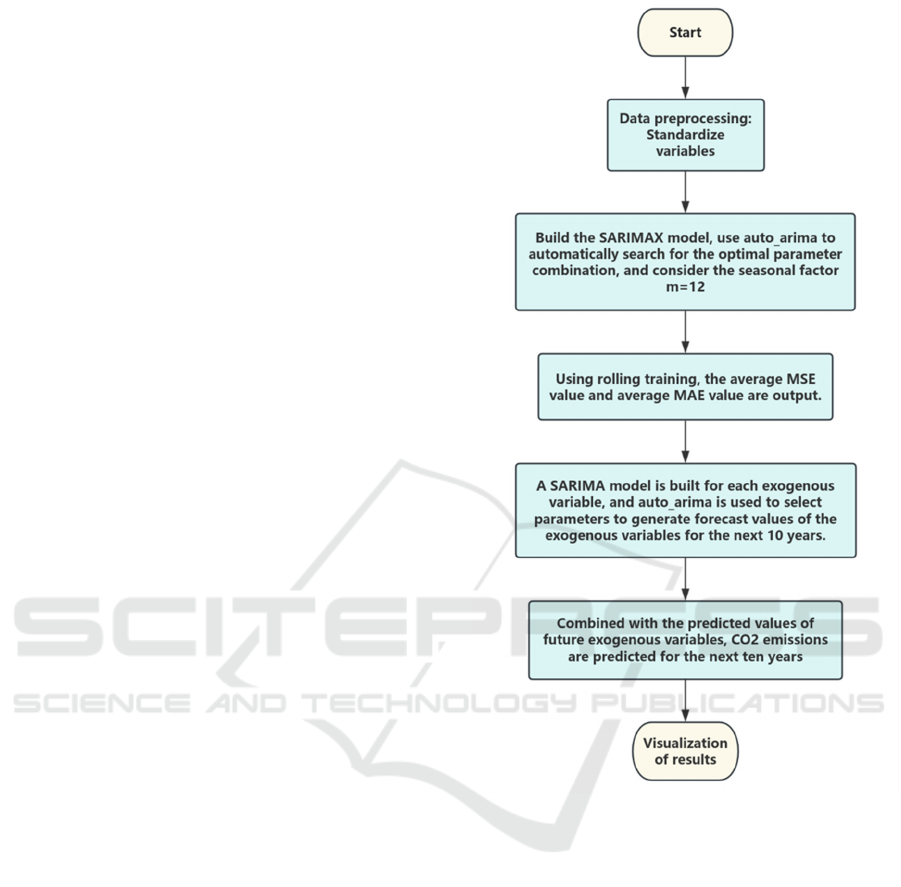
The modeling and prediction of the SARIMAX
model includes six steps, as depicted in Figure 1:
Figure 1: SARIMAX prediction model flow chart (Picture
credit: original).
2.3 GRU Model
The GRU model is a variant model based on the
LSTM model architecture. It updates and resets the
hidden state through a gating mechanism to balance
historical information and new information currently
input, thereby dynamically controlling the flow of
information. Compared with the complex gating
mechanism of the LSTM model, GRU optimizes the
association between the input gate and the forget gate
in the LSTM into an update gate (Mahjoub, Chrifi-
Alaoui, Marhic, et al, 2022). Therefore, the gated
recurrent unit of GRU has only two gates, namely the
reset gate and the update gate. The update gate (Z
)
determines the extent to which the new hidden state
is updated to the current hidden state, that is, how
ICDSE 2025 - The International Conference on Data Science and Engineering
334
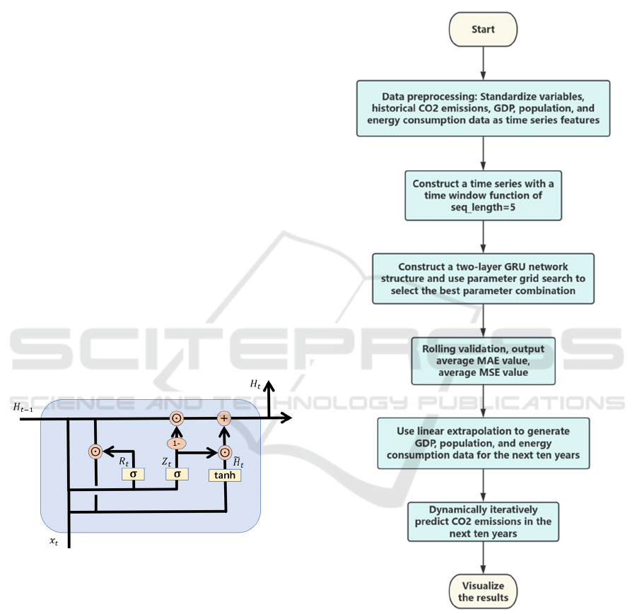
much new information is updated. The reset gate (R
)
determines the degree of forgetting historical
information, that is, it determines the degree to which
the hidden state at the previous moment can affect the
current hidden state. A candidate hidden state (H
) is
a temporarily generated hidden state that combines
the current input information with some historical
information. Finally, the candidate hidden state and
the previous hidden state are combined via the update
gate to calculate the hidden state, and this resultant
hidden state is then fed as input to the next gated unit
in the sequence.
The expression of the gate unit is:
Z
=σW
∙
H
,x
+a
(7)
R
=σW
∙
H
,x
+a
(8)
H
=tanhW
∙R
⨀H
,x
+a
(9)
H
=1Z
⨀H
+Z
⨀H
(10)
Where x
is the current input, H
is the hidden
state at the previous moment, W
,W
,W
are
weight parameters, a
,a
,a
is the bias
parameter, σ is the sigmoid function, the symbol ⨀
represents the Hadamard product, and tanh is the
nonlinear activation function.
One of the gate unit processes is shown in Figure
2:
Figure 2: GRU model gate unit flow chart (Picture credit:
original).
According to studies, the GRU model performs
similarly to the LSTM model in many situations.
However, GRU speeds up training by reducing the
LSTM's input, forget, and output gates to an update
gate and a reset gate. More importantly, the direct
transmission of the GRU hidden state makes the
gradient propagation path more direct, which can
effectively alleviate problems such as gradient
disappearance or explosion (
Shiri, Perumal,
Mustapha, et al, 2024)
. In addition, the LSTM
model is better at processing very long sequences,
and the GRU model requires relatively less
summarized data, so it is more suitable for
predicting CO
2
emissions based on annual data.
The modeling and prediction of the GRU model
mainly includes 7 steps, as shown in Figure 3:
Figure 3: GRU prediction model flow chart (Picture credit:
original).
3 RESULTS
3.1 Driving Factors
Among the 27 EU member states, the three driving
factors of most member states passed the p-value test
A Comparative Study and Forecast of Carbon Dioxide Emissions in EU Countries over the Next Decade Using SARIMAX and GRU Models
335
based on the linear regression model, indicating that
they have a significant impact on CO
2
emissions.
All three factors of Malta failed the p-value test,
so the SARIMA model was used to model it without
adding exogenous variables. When predicting with
the GRU model, only CO
2
historical data was used as
the characteristic variable, and no other variables
were added.
The population and GDP factors of Croatia,
Finland, Italy, Luxembourg, and the Netherlands did
not pass the p-value test, so only energy consumption
was used as an exogenous variable and eigenvector in
the prediction.
The GDP factors of Estonia, Latvia, Lithuania,
and Slovenia did not pass the p-value test, so energy
consumption and population size were used as
exogenous variables and eigenvectors to participate
in the prediction.
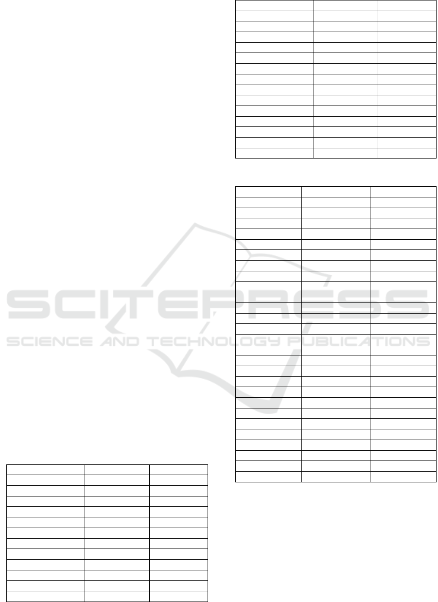
3.2 Average MAE and Average MSE
As shown in the results in Table 1 and Table 2, for
most EU countries, the average MSE and average
MAE indicators of the SARIMAX model and the
GRU model are close to 0, which indicates that both
the average absolute error and the average square
error between the two models' actual values and their
predictions are minor. The performance of both
models is relatively good, and the prediction of CO
2
emissions is relatively reliable. The SARIMAX
model's average MSE and average MAE values are
less than the GRU model's, suggesting that there are
fewer outliers in the training results of the SARIMAX
model, and the average prediction deviation under the
stationarity assumption is also smaller than that of the
GRU model. Compared with the GRU model, it
shows good time series processing capabilities and is
better suited for forecasting CO
2
emissions in EU
member states.
Table 1: Average MAE value of the two models.
Avera
g
e MAE SARIMAX GRU
Austria 0.08463 0.14220
Belgiu
m
0.09486 0.14692
Bulgaria 0.02233 0.08012
Croatia 0.11287 0.09653
C
yp
rus 0.04145 0.08090
Czechia 0.02292 0.05710
Denmar
k
0.02962 0.07477
Estonia 0.03359 0.07863
Finlan
d
0.03627 0.15370
France 0.04181 0.04479
German
y
0.02376 0.05496
Greece 0.04687 0.06994
Hun
g
ar
y
0.01781 0.04249
Irelan
d
0.02324 0.11046
Ital
y
0.02834 0.10906
Latvia 0.03057 0.01763
Lithuania 0.02621 0.01054
Luxembour
g
0.03029 0.10679
Malta 0.13111 0.08099
Netherlands 0.05900 0.18846
Polan
d
0.01478 0.10907
Portu
g
al 0.06811 0.14421
Romania 0.03057 0.01830
Slovakia 0.01816 0.07619
Slovenia 0.05058 0.08561
Spain 0.04226 0.10774
Sweden 0.02416 0.04887
Table 2: Average MSE value of the two models.
Avera
g
e MSE SARIMAX GRU
Austria 0.01153 0.02467
Belgiu
m
0.01190 0.02612
Bulgaria 0.00087 0.00853
Croatia 0.02142 0.01159
C
yp
rus 0.00274 0.01191
Czechia 0.00069 0.00382
Denmar
k
0.00116 0.00680
Estonia 0.00126 0.01123
Finlan
d
0.00208 0.02906
France 0.00211 0.00301
German
y
0.00085 0.00638
Greece 0.00281 0.00862
Hungary 0.00043 0.00205
Irelan
d
0.00118 0.02289
Ital
y
0.00106 0.01598
Latvia 0.00197 0.00049
Lithuania 0.00083 0.00026
Luxembourg 0.00207 0.01582
Malta 0.03242 0.01279
Netherlands 0.00499 0.05676
Polan
d
0.00049 0.01407
Portu
g
al 0.00632 0.03379
Romania 0.00115 0.00049
Slovakia 0.00052 0.00660
Slovenia 0.00411 0.00887
S
p
ain 0.00273 0.02126
Sweden 0.00086 0.00459
3.3 Forecast Results of Carbon Dioxide
Emissions in the Next Ten Years
The prediction results are shown by taking Germany,
France and Poland, three countries with high
emissions in 2022, as examples. The results show that
the SRIMAX and GRU models forecast similar trends
for the majority of countries. The SARIMAX model
can better fit the fluctuations in historical data. In
ICDSE 2025 - The International Conference on Data Science and Engineering
336
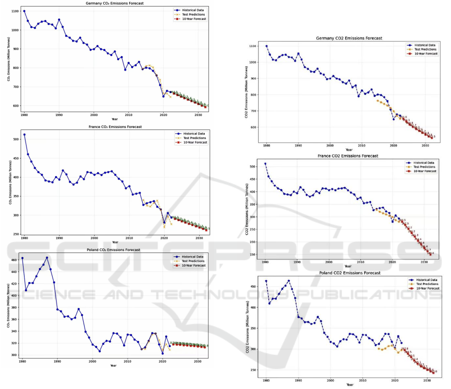
contrast, the GRU model fits the training history data
less well than the SARIMAX model and performs
poorly when dealing with outliers in historical data.
Figure 4: SARIMAX model prediction results (Picture
credit: original).
It is speculated that the possible reason for the
error between the training data and the real data is that
the model cannot capture the intervention of policy
factors and there are fewer driving factors. In addition,
it is speculated that the possible reason why the
SARIMAX model has a higher fitting accuracy for
historical data with large fluctuations than the GRU
model is that the SARIMAX model, as a traditional
statistical model, is more suitable for small sample
time series, while GRU, as a neural network model,
requires more data to capture complex patterns. The
SARIMAX model captures cyclical changes through
seasonal_order, which may have a more significant
advantage in long-term trend forecasting. The
SARIMAX model explicitly quantifies the impact of
exogenous variables on CO2 through differentials,
which is highly interpretable, while the GRU model
inputs feature variables into a black box network,
which may result in the inability to effectively
separate the independent impact of driving factors.
Figure 5: GRU model prediction results (Picture credit:
original).
Although the prediction trends of CO
2
emissions
for most EU countries based on the SARIMAX model
and the GRU model are the same, there are some
countries with opposite prediction trends. It is
speculated that the possible reason is that the
SARIMAX model predicts a downward trend when
CO
2
emissions show a non-monotonic trend of first
increasing and then decreasing due to the fixed
difference order, while the GRU model may have
captured the recovery signal after the inflection point.
The GRU model generates future features through
linear extrapolation and has poor adaptability to
A Comparative Study and Forecast of Carbon Dioxide Emissions in EU Countries over the Next Decade Using SARIMAX and GRU Models
337

changes in nonlinear feature vectors (such as sudden
population growth). Figure 4 and Figure 5 show that
the SARIMAX model and the GRU model differ in
predicting the rate of decline in CO
2
emissions. It is
speculated that the possible reason is that some
countries have quickly turned to renewable energy,
resulting in a CO
2
decline rate that is higher than the
historical law. At the same time, the SARIMAX
model relies on historical data and may underestimate
the speed of emission reduction. If the GRU model
captures recent mutation signals, it may predict a
more radical decline.
4 DISCUSSIONS
This study shows that the CO
2
emissions of 17 of the
27 EU member states are declining in the trends
predicted by both models, indicating that the
measures and policies taken by the EU have
effectively reduced CO
2
emissions. The rate of
decline in CO
2
emissions in most countries has
increased significantly since 2005, presumably
because the EU carbon emissions trading system
established in 2005 has been effective in reducing
greenhouse gas emissions. At the same time, CO
2
emissions in EU countries also dropped significantly
after 2018. It is speculated that the possible reason is
that the revision of the Renewable Energy Directive
in 2018 effectively improved energy efficiency,
resulting in a significant drop in CO
2
emissions. The
series of measures taken by the EU have achieved
remarkable results in reducing CO
2
emissions.
Therefore, other countries should actively learn from
its successful experience and strengthen international
cooperation. The EU should actively provide
corresponding assistance and support, give full play
to its leading role, and help advance the global
climate governance process to achieve the goals set
out in the Paris Agreement.
Although the average MAE and average MSE
values of the SARIMAX model and the GRU model
are close to 0, they can still be further improved. The
SARIMAX model is more reliable in predicting
countries with relatively stable historical trends,
while GRU is good at capturing mutation signals to
make predictions, so a GRU-SARIMAX hybrid
model can be constructed to predict CO
2
emissions.
At the same time, this study uses monthly data. If
high-precision predictions of CO
2
emissions for a
specific country are required, it is recommended to
use monthly and quarterly data on CO
2
emissions to
better capture historical trends and mutation nodes. It
is difficult to find the same driving factors for CO
2
emissions for the entire EU countries. Therefore, this
study only uses three driving factors to make
predictions for the countries. If a specific country is
studied, additional driving factors can be added based
on the country's national conditions to better fit the
historical data curve and improve model
performance.
5 CONCLUSIONS
Through the study and prediction of CO
2
emissions in
EU countries in the next 10 years, the SARIMAX
model's average MAE and average MSE values are
found to be lower than the GRU model's.
Consequently, the SARIMAX model is more suited
for forecasting CO
2
emissions in EU countries in this
study. The possible reason is that the SARIMAX
model's superiority for small sample time series
prediction. At the same time, the study found that CO
2
emissions in most EU countries will continue to
decline in the next 10 years. Therefore, it is
anticipated that the European Climate Law's target of
reducing greenhouse gas emissions by at least 55%
by 2030 in comparison to 1990 will be met. The main
contribution of this study is the prediction of carbon
emissions of 27 EU countries in the next 10 years,
proving that the policies formulated by the EU have
achieved significant results in emission reduction,
and contrasting the GRU prediction model's
performance in a small sample scenario with that of
the SARIMAX prediction model. This study provides
a reference for other scholars when selecting a small
sample CO
2
emission prediction model. In addition,
other major CO
2
emitting countries can learn from the
EU's economic transformation approach and
measures and policies such as improving energy
efficiency to promote the realization of the goals of
the Paris Agreement, thereby alleviating major
problems facing society today, such as climate
change, environmental degradation and resource
depletion. As described in this study, the SARIMAX
model and the GRU model each have their own
advantages. In future studies, a hybrid model GRU-
SARIMAX can be proposed to improve prediction
accuracy and model performance.
REFERENCES
Cifuentes-Faura, J., 2022. European Union policies and
their role in combating climate change over the years.
Air Quality, Atmosphere & Health, 15(10), 1333–1340.
Springer. Berlin.
ICDSE 2025 - The International Conference on Data Science and Engineering
338

Hodson, T. O., 2022. Root-mean-square error (RMSE) or
mean absolute error (MAE): when to use them or not.
Geoscientific Model Development, 15(14), 5481–5487.
European Geosciences Union. Göttingen.
Jin, Y., Sharifi, A., Li, Z., Chen, S., Zeng, S., & Zhao, S.,
2024. Carbon emission prediction models: A review.
Science of the Total Environment, 927, 172319.
Elsevier. Amsterdam.
Li, X., & Zhang, X., 2023. A comparative study of
statistical and machine learning models on carbon
dioxide emissions prediction of China. Environmental
Science and Pollution Research, 30, 117485–117502.
Springer. Berlin.
Mahjoub, S., Chrifi-Alaoui, L., Marhic, B., & Delahoche,
L., 2022. Predicting Energy Consumption Using
LSTM, Multi-Layer GRU and Drop-GRU Neural
Networks. Sensors, 22(11), 4062. MDPI. Basel.
Radmehr, R., Henneberry, S. R., & Shayanmehr, S., 2021.
Renewable Energy Consumption, CO₂ Emissions, and
Economic Growth Nexus: A Simultaneity Spatial
Modeling Analysis of EU Countries. Structural Change
and Economic Dynamics, 57, 13-27. Elsevier.
Amsterdam.
Shiri, F. M., Perumal, T., Mustapha, N., & Mohamed, R.,
2024. A Comprehensive Overview and Comparative
Analysis on Deep Learning Models: CNN, RNN,
LSTM, GRU. Journal on Artificial Intelligence, 6(1),
301–360. Tech Science Press. New York.
United Nations Environment Programme, 2023. Emissions
Gap Report 2023: Broken Record – Temperatures hit
new highs, yet world fails to cut emissions (again).
United Nations Environment Programme. Nairobi.
ISBN: 978-92-807-4098-1.
Wen, T., Liu, Y., Bai, Y. H., & Liu, H. Y., 2023. Modeling
and forecasting CO2 emissions in China and its regions
using a novel ARIMA-LSTM model. Heliyon, 9(11),
1241-1251. 2nd edition.
Zhao, X. F., & Li, Y. L., 2021. Analysis of influencing
factors on China's CO₂ emissions prediction based on
LSTM model. China Market, (22), 15-16. Beijing.
A Comparative Study and Forecast of Carbon Dioxide Emissions in EU Countries over the Next Decade Using SARIMAX and GRU Models
339
