A Study on Stock Price Forecasting of Semiconductor Industry in

Technology Sector Based on ARIMA Modeling:

NVIDIA Corporation (NVDA) as an Example

Zhibin Zhao

College of Statistics and Mathematics, Shandong University of Finance and Economics Jinan, Shandong, China

Keywords: Semiconductor Industry, Stock Price Forecasting, ARIMA Model, Time Series Analysis, Investment Decision

Making.

Abstract: Given how quickly the world economy is growing and how the semiconductor industry is at the forefront of

science and technology, changes in its stock price have a big impact on businesses and investors. In order to

assist investors in better understanding market dynamics, this article forecasts the semiconductor industry's

stock price using the Autoregressive Integrated Moving Average (ARIMA) model. A semiconductor

company's daily closing price data from 2022 to 2025 is chosen for the study, and the ARIMA model is used

for modeling and forecasting. The model's performance is assessed using the mean square error and the

average absolute error. The findings demonstrate that the ARIMA model fits and forecasts semiconductor

stock values more accurately, making it a useful tool for investors. In addition to adding to the body of

empirical research on stock price prediction, this study offers theoretical justification for investing choices in

related domains.

1 INTRODUCTION

Stock price forecasting is an important research

direction in finance, and the Autoregressive

Integrated Moving Average(ARIMA)model is widely

used for its good ability to handle non-stationary

series (Huang, 2023). However, most of the existing

studies focus on traditional industries, and the

applicability of the ARIMA model to the

semiconductor industry, which is highly volatile and

strongly cyclical, remains to be explored. As the core

of modern technology, the semiconductor industry's

stock price volatility is affected by multiple factors

such as corporate operations, macroeconomics,

market sentiment and technological breakthroughs,

and accurate forecasting is significant for investors

and corporate strategic planning. In recent years, the

ARIMA model has provided a new perspective for

studying semiconductor stock prices, but its

effectiveness in this field needs to be further verified.

In recent years, scholars have explored stock price

forecasting in depth through different methods. For

example, Huang verified the robustness of the

https://orcid.org/0009-0006-3431-7083

ARIMA model in stock price forecasting through

empirical research with the ARIMA model as the

core, but the object of his research did not involve the

semiconductor industry (Huang, 2023). Yi Zhang

(2022) proposed a combination model of ARIMA and

Attention-based Long Short Term Memory(AT-

LSTM), and the outcomes demonstrated how well the

hybrid model can raise prediction accuracy, but its

research is still limited to traditional manufacturing

stocks (Zhang, 2022). In addition, Wu et al. ARIMA-

based short-term forecasting framework provides a

technical reference for this paper, but it fails to take

into account the specificity of the semiconductor

industry (Wu & Wen, 2016).

Overall, although the existing literature verifies

the universality of the ARIMA model, there is still a

gap in the research on stock price forecasting for the

semiconductor sector.

This paper's goal is to investigate the performance

of semiconductor stocks in short-term price

forecasting by constructing an ARIMA model and

combining its high-frequency data characteristics.

Zhao, Z.

A Study on Stock Price Forecasting of Semiconductor Industry in Technology Sector Based on ARIMA Modeling: NVIDIA Corporation (NVDA) as an Example.

DOI: 10.5220/0013685600004670

Paper published under CC license (CC BY-NC-ND 4.0)

In Proceedings of the 2nd International Conference on Data Science and Engineering (ICDSE 2025), pages 235-241

ISBN: 978-989-758-765-8

235

There are four sections to this article. The

introduction, which presents the research

background, previous research methods and the

research purpose of this paper, is the first section; the

second part is the data and methodology, which

describes in detail the data sources, data

preprocessing and model principles; the third part is

the empirical analysis, which demonstrates and

analyzes the experimental results; and the fourth part

is the conclusion, which summarizes the findings of

the study and puts forward the future research

direction.

2 DATA AND METHODS

2.1 Data Collection and Analysis

In this paper, the daily closing price data of a

semiconductor company from January 1, 2022, to

January 31, 2025, are selected from the financial data

platform. The data sample has a total of 751

observations with a time span of 3 years (Guo&Wang

2023). The overall trend of the data shows some

volatility, reflecting the complexity of stock prices in

the semiconductor industry. The basic descriptive

statistics of the data are shown in Table 1.

Table 1: Closing Price Descriptive Statistics.

Statistic Min 1st Qu. Median Mean 3rd Qu. Max Va

Sd.

Prices 11.23 19.57 42.69 57.03 90.41 149.43 1915.387 43.76514

2.2 Data Preprocessing

The accuracy of stock price prediction is highly

dependent on the quality and applicability of data. In

view of the high-frequency trading characteristics and

volatility features of stocks in the semiconductor

field, the data preprocessing process in this study

mainly includes the following steps.

First, the historical daily frequency trading data

(opening price, closing price, volume, etc.) of a

leading stock in the semiconductor industry are

selected, and the data are integrated through Python's

panda's library. For abnormal values (e.g., extreme

rise and fall), the box plot method is used to identify

and eliminate them, and missing values are filled in

by the linear interpolation method to ensure data

continuity.

Second, semiconductor stock price series are

usually trending and non-stationary, and their

stationarity should be verified by the Augmented

Dickey-Fuller Test(ADF test).

The ADF test's initial hypothesis (H0) states that

the time series has a unit root, or is non-stationary,

whereas the alternative hypothesis (H1) states that the

time series has no unit root, or is stationary. To

identify the ideal lag order, the test typically employs

an information criterion, such as the Bayesian

Information Criterion (BIC) or the Akaike

Information Criterion (AIC). After determining the

model parameters using least squares, the ADF

statistic is then calculated. Additionally, the critical

value and the ADF statistic are compared. If the ADF

statistic is less than the critical value, the original

hypothesis is rejected and the series is considered

smooth (Wang, 2021). At the same time, the p-value

can also be calculated for judgment, and if the p-value

is less than the significance level (e.g., 0.05), the

original hypothesis is rejected. If the series is not

smooth, the trend term is eliminated by the difference

operation (i.e., the “I” part of ARIMA) until the

series meets the smoothness requirement.

Finally, the processed price series are Z-score

normalized to remove the magnitude difference in

order to improve the model's rate of convergence.

2.3 Principle of the Model

2.3.1 ARIMA Model

The ARIMA model is a classical time series

forecasting method whose core consists of the

following three components.

First is Autoregressive (AR). In this part, the

linear combination of historical observations is

utilized to forecast future values, the order p indicates

the dependent historical step, and the model

expression is shown in Equation (1) (Wang, 2024) .

𝛸



=𝑐+∅



𝛸



+∅



𝛸



+⋯+∅



𝛸



+𝜖







where ∅ is the autoregressive coefficient and is

white noise.

The second is Difference (I). This section

addresses trend and seasonal fluctuations by using

differencing to transform a non-stationary series into

a stationary series.

Third is the Moving Average (MA). This part,

corrects the forecast value based on a linear

combination of historical forecast errors, with order q

reflecting the range of influence of the error term, and

ICDSE 2025 - The International Conference on Data Science and Engineering

236

the expression is shown in Equation (2) (Wang,

2024).

𝑋



=𝜇+𝜖



+𝜃



𝜖



+𝜃



𝜖



+⋯+𝜃



𝜖







Where 𝜃 is the moving average coefficient.

2.3.2 Parameter Determination and Model

Optimization

First, Autocorrelation coefficient(ACF) and Partial

autocorrelation coefficient(PACF) plots are plotted

for model parameter analysis, and the values of p and

q are preliminarily determined by the autocorrelation

function and partial autocorrelation function plots(Li,

2022). The principle of model parameter

identification is shown in Table 2.

Table 2: Model parameter identification table.

ACF PACF Model

trailing tail

p-step

trailin

AR(p)Model

q-order

truncation

truncation MR(q)Model

trailing tail trailing tail

ARMA(p，q)

Model

Second, the grid search method. Combining the

AIC or BIC criterion, traverse different parameter

combinations (p, d, q) and select the optimal model

that minimizes the information criterion.

Third, residual test. The Ljung-Box test is

performed on the model residuals to ensure that they

conform to the white noise characteristics and to

avoid under-extraction of information. The Ljung-

Box test's main objective is to determine if a time

series has substantial autocorrelation by summing the

series' autocorrelation coefficients. A chi-square

distribution with degrees of freedom m is obeyed by

its test statistic, Q. The original hypothesis of the test

(H0) is that the individual values of the time series are

independent (i.e., there is no autocorrelation) and the

series is white noise; the alternative hypothesis (H1)

is that the individual values of the time series are not

independent and that there is autocorrelation. The test

begins with the selection of the appropriate lag order,

and the choice of the end of the lag is usually based

on the sample size and analytical needs. Generally,

the lag order can be set to 1/4 of the length of the

series. Second, calculate the test statistic. The Ljung-

Box statistic Q, which measures the autocorrelation

of the series over multiple lags, is calculated

according to the formula.The initial hypothesis is

disproved and the series is deemed autocorrelated if

the computed Q value translates into a p-value below

the significance level, which is typically 0.05.

3 EMPIRICAL ANALYSIS

3.1 Data Selection

Studying the trajectory of the closing price of

NVIDIA's stock is crucial because of the company's

representative position in the semiconductor sector on

the US stock exchange. In this paper, the closing price

of NVIDIA stock from January 1, 2022, to January

31, 2025, is selected as the original data (a total of

751) for time series analysis(Qi, 2021).

3.2 Smoothness Test and Difference

Processing

This study examines the smoothness of 751 closing

price data points from NVIDIA's trading days during

the previous three years and the smoothness of the

raw data is observed by plotting the ACF chart and

PACF chart, and the results are shown in Figures 1

and 2 below.

The autocorrelation coefficient in the ACF plot

(Figure 1) is 1 at lag 0, which is due to the perfect

correlation of any series with itself. As the lag

increases, the autocorrelation coefficient decreases

slightly but still remains at a high level. This indicates

that NVIDIA stock price has significant

autocorrelation in the short or long run.

However, in the PACF plot (Figure 2), the biased

autocorrelation coefficient is 1 at lag 0; at lag 1,there

is considerable autocorrelation at lag 1, as indicated

by the biased autocorrelation coefficient being

significantly larger than 0. As the lag period

increases, the partial autocorrelation coefficient

decreases rapidly and approaches 0 after lag 2. This

indicates that there is significant autocorrelation in

NVIDIA's stock price in the short term (lag 1), but no

significant autocorrelation in the longer lag period.

In summary, Figure 1 and Figure 2 show that

NVIDIA stock price has significant autocorrelation in

the short term (lag 1) and no significant

autocorrelation in the longer lag. Thus, this property

suggests that the NVIDIA stock price data has some

predictability in the short run, but exhibits

randomness over longer periods of time, and the

series is considered to be unstable.

A Study on Stock Price Forecasting of Semiconductor Industry in Technology Sector Based on ARIMA Modeling: NVIDIA Corporation

(NVDA) as an Example

237

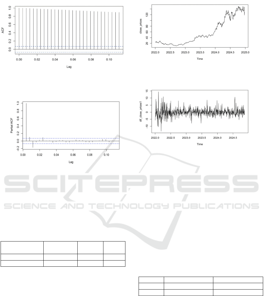
Figure 1: NVIDIA Stock Closing Price ACF Chart. (Picture

credit: Original)

Figure 2: NVIDIA Stock Closing Price PACF Chart.

(Picture credit: Original)

In the meantime, the raw data is subjected to an

ADF test in this study; the outcomes are displayed in

Table 3. Again, the series is not considered smooth

because the p-value of 0.4425 is more than the

significance level of 0.05, as indicated in Table 3.

Table 3: ADF test result table.

DATA

Dickey-

Fulle

Lag

orde

value

rices -2.3209 9 0.4425

diff

rices -8.48 9 0.01

The series is processed using the difference

technique to get a smooth series. The differenced

series is subjected to the ADF smoothness test, and

Table 3 displays the findings: Since the p-value is

0.01, which is less than 0.05, the differenced series

can be regarded as smooth. The smoothness of the

time series can also be observed by plotting the time

series. As shown in Figure 3, the original series has

an obvious upward trend; while in Figure 4, the first-

order differenced series has no obvious trend or

periodicity, indicating that the time series data have

been stabilized after the first-order differencing

process.

Figure 3: Differential Front Sequence Diagram. (Picture

credit: Original)

Figure 4: Differential Sequence Diagram. (Picture credit:

Original)

3.3

White Noise Test

After the smoothness test the first-order difference

sequence already has a smoothness, in addition to

this, also need to carry out a white noise test on the

smooth sequence. There are three general white noise

tests: autocorrelation diagram, Ljung-Box test and

Box-Pierce test. This paper chooses the Ljung-Box

test for white noise, and calculates the lagged 6th and

12th order Ljung-Box statistic and p-value, the results

are shown in Table 4 below: p-value is less than 0.05,

and it can be assumed that the sequence of the first-

order difference is a non-white noise sequence.

Table 4: Ljung-Box test results table.

X-s

uare

-value

6 23.394 0.0006747

12 31.122 0.001887

3.4

Model Ordering and Parameter

Estimation

The model order, or p and q in an ARIMA (p,d,q)

model, may often be found in two methods.The first

method is to calculate the ACF and the PACF, and to

choose the appropriate p and q values to fit the model

according to the “trailing” and “truncated” nature of

the coefficients(Liu, 2021) .

ICDSE 2025 - The International Conference on Data Science and Engineering

238

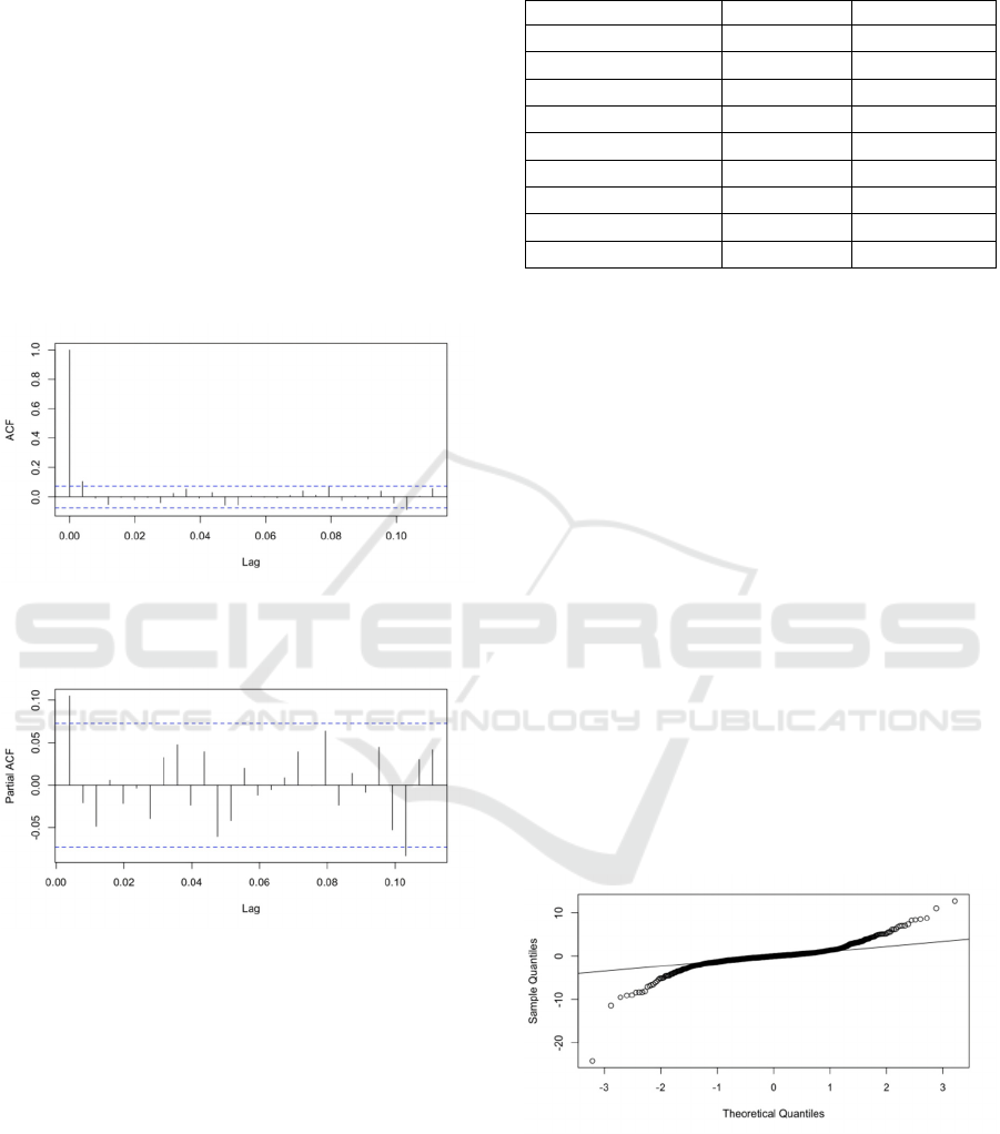
In the ACF plot (Figure 5), the autocorrelation

coefficient decreases rapidly after lag 1 and

approaches zero at most of the lags and is within the

significance bounds, showing the 1st order tailing

phenomenon. In the PACF plot (Figure 6), the biased

autocorrelation coefficient is 1 when the lag is 0. As

the lag increases to the 1st order, the biased

autocorrelation coefficient decreases rapidly and

approaches 0. Although it fluctuates at different lags,

most of the values are within the significance bounds

(blue dashed line), presenting a 1st order truncated

tail phenomenon.

Therefore, the time series model used to forecast

this company's stock price is the ARIMA (1, 1, 1)

model.

Figure 5: NVIDIA Post-Differential Stock Closing Price

ACF Chart. (Picture credit: Original)

Figure 6: NVIDIA Post-Differential Stock Closing Price

PACF Chart. (Picture credit: Original)

In addition to this, this paper uses AIC and BIC

criteria for model ordering. In R, the values of p, and

q are specified as 1, 2, and 3, respectively, and the

AIC and BIC values of the respective order models

are calculated, and the results are shown in Table 5

below. The conclusions obtained from this method

are consistent with the first one, so ARIMA (1, 1, 1)

is finally determined to fit the trend of stock closing

price changes.

Table 5: Results of AIC and BIC values for ARIMA model

of each order.

ARIMA AIC BIC

(1，1，1)

3464.29 3482.770

(1，1，2)

3466.62 3485.102

(1，1，3)

3469.97 3493.068

(2，1，1) 3466.65 3485.135

(2，1，2) 3468.00 3491.104

(2，1，3) 3467.44 3495.159

(3，1，1) 3468.14 3491.238

(3，1，2)

3467.24 3494.959

(3，1，3)

3499.11 3481.447

For ARIMA (1, 1, 1) to be estimated, the model

fit equation is shown in equation (3). Where the drift

term (drift) is a constant term that indicates the long

term trend or linear trend in the time series data. The

drift term in this model has a value of 0.1374,

meaning that, in the absence of any other influencing

variables, the time series value will progressively rise

by 0.1374 units over time.



0.8418  0.8418B





1  0.7602B



+ 0.1374





3.5

Residual Test

There are two components to the fitted model's

residual test, which are normality test and residual

analysis. A Q-Q diagram of the residuals is plotted as

part of the normality test to determine whether the

residuals are normal. If the residuals are normally

distributed, the sample quartiles should fall roughly

on a straight line. As can be seen in Figure 7, most of

the points are on a straight line, but there are some

deviations at the ends, especially around -3 and 3.

Overall the residuals can be considered normal.

Figure 7: Residual Q-Q Plot. (Picture credit: Original)

Residual analysis starts with three parts: first, a

plot of the residuals in time (Figure 8 top left). The

residuals should fluctuate up and down around zero,

with no apparent trend or periodicity. As can be seen

from the graph, the residuals fluctuate roughly around

A Study on Stock Price Forecasting of Semiconductor Industry in Technology Sector Based on ARIMA Modeling: NVIDIA Corporation

(NVDA) as an Example

239

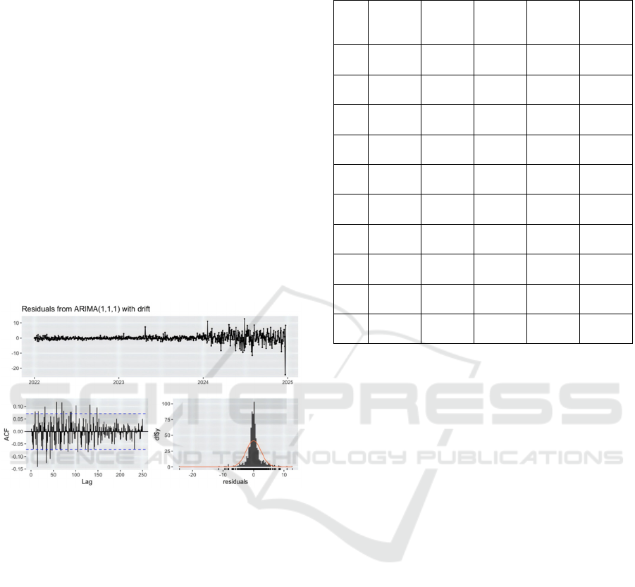
zero, which is in line with the requirements overall,

but there are large fluctuations in 2024 and 2025, and

further examination of the data for these time periods

may be needed.

Second, the autocorrelation function (ACF) plot

(Figure 8 bottom left). The ACF plot is used to check

the autocorrelation of the residuals. The blue dashed

lines indicate the significance bounds, and residuals

within these bounds indicate no significant

autocorrelation. As can be seen from the figure, there

is no discernible autocorrelation in the residuals

because the majority of them fall under the

significance boundaries.

Third, the histogram of the residuals (Figure 8

bottom right). The histogram is used to examine the

distribution of the residuals. The red curve indicates

the fit of the normal distribution. The residuals'

distribution is approximately symmetrical, as the

image illustrates, although there are occasional

departures from the usual distribution, particularly

toward the ends.

Figure 8: Plot of residual test results. (Picture credit:

Original)

3.6

Model Forecasting

The model is used to analyze the short-term price

prediction of the stock and predict the closing price of

the stock for the next 10 trading days(Yu, Cai, & Xia,

2015). The results are shown in Table 6. From

126.7064 on January 29, 2025, to 129.2847 on

February 7, 2025, the overall trend is upward, but

with slight decreases on February 2nd and February

4th. At the same time, the width of both the 80% and

95% confidence intervals increased as the dates

progressed, indicating an increase in forecast

uncertainty.

Table 6: Results of stock closing price prediction for the

next 10 trading days in 2025.

Dat

Point

Foreca

Lo 80 Hi 80 Lo 95 Hi 95

1.2

126.70

123.59

129.81

121.94

131.46

1.3

128.88

124.65

133.10

122.41

135.34

1.3

127.30

122.07

132.52

119.31

135.29

2.1

128.88

122.91

134.85

119.75

138.01

2.2

127.80

121.10

134.50

117.55

138.05

2.3

128.96

121.65

136.27

117.78

140.14

2.4

128.24

120.33

136.15

116.14

140.34

2.5

129.10

120.67

137.54

116.20

142.00

2.6

128.63

119.67

137.58

114.93

142.33

2.7

129.28

119.85

138.71

114.86

143.70

This gives investors some food for thought, and

this article gives the following six takeaways.

First, the overall trend is upward, which could

indicate that the market is optimistic about NVIDIA

stock. Investors may consider buying when prices are

low with a view to taking profits when prices rise.

Second, the width of the confidence interval has

increased, indicating an increase in forecast

uncertainty. Investors should be aware of the

possibility of greater price volatility in the future and

the need for good risk management.

Third, investors can use confidence intervals to

assess potential risks and rewards. For example, if

investors are willing to take higher risks, they may

consider buying near the lower limit of the confidence

interval with a view to obtaining higher returns.

In conclusion, while forecasts provide a useful

starting point, investors should take into account their

risk tolerance, investment objectives and market

research in making their final investment decisions.

4 CONCLUSIONS

This gives investors some food for thought, and this

article gives the following six takeaways.

First, the overall trend is upward, which could

indicate that the market is optimistic about NVIDIA

ICDSE 2025 - The International Conference on Data Science and Engineering

240

stock. Investors may consider buying when prices are

low with a view to taking profits when prices rise.

Second, the width of the confidence interval has

increased, indicating an increase in forecast

uncertainty. Investors should be aware of the

possibility of greater price volatility in the future and

the need for good risk management.

Third, investors can use confidence intervals to

assess potential risks and rewards. For example, if

investors are willing to take higher risks, they may

consider buying near the lower limit of the confidence

interval with a view to obtaining higher returns.

In conclusion, while forecasts provide a useful

starting point, investors should take into account their

risk tolerance, investment objectives and market

research in making their final investment decisions.

REFERENCES

Guo, G., & Wang, S. 2023. Stock price prediction based on

gray theory and ARIMA model. Journal of Henan

Institute of Education (Natural Science Edition),

32(02), 22–27.

Huang, M. 2023. Empirical research on stock price

forecasting based on ARIMA model. Neijiang Science

and Technology, 44(03), 61–62.

Li, Y. 2022. Short-term forecasting of stock price based on

ARMA model—Taking Gujing Gongjiu stock as an

example. Journal of Shanxi Finance and Taxation

College, 24(01), 25–30.

Liu, J. 2021. The application of ARMA model in stock price

forecasting—Taking Gree Electric as an example.

China Management Informatization, 24(11), 153–155.

Qi, T. 2021. Stock price prediction based on gray model and

ARIMA model. Computer Age, 10, 83–85, 89.

Wang, Y. 2021. Analysis and prediction of stock price

based on ARMA model. Productivity Research, 9, 124–

127.

Wang, Z. 2024. Research on stock price prediction model

and trading strategy based on deep learning.

Guangdong Technology Normal University.

Wu, Y., & Wen, X. 2016. Short-term stock price

forecasting based on ARIMA model. Statistics and

Decision Making, 23, 83–86.

Yu, H., Cai, J., & Xia, H. 2015. Application of ARIMA

model in stock price forecasting. Economist, 11, 156–

157.

Zhang, Y. 2022. Stock price prediction based on ARIMA

and AT-LSTM combination model. Computer

Knowledge and Technology, 18(11), 118–121.

A Study on Stock Price Forecasting of Semiconductor Industry in Technology Sector Based on ARIMA Modeling: NVIDIA Corporation

(NVDA) as an Example

241