Machine Learning Solutions for Heart Disease Diagnosis: Model

Choices and Factor Analysis

Hao Rui

Zhejiang University - University of Illinois Urbana-Champaign Institute, Zhejiang University, Jiaxing, Zhejiang, China

Keywords: Machine Learning, Model Training, Heart Disease Diagnosis.

Abstract: The prediction of heart disease diagnosis is of paramount importance since it is one of the leading causes of

death nowadays. Yet accurately identifying and monitoring the factors relative to heart diseases pose

significant challenges. Traditional visual survey methods are time-consuming, often hampered by the lack of

data exchange among hospitals and individual doctors, and may not provide real-time data crucial for effective

prevention strategies. Machine learning (ML) technologies have become increasingly potent instruments in

the diagnosis of diseases in recent years. In this project, several models were investigated. A complete set of

data gathered from Long Beach V, Cleveland, Hungary, and Switzerland was utilized. This data set, which

encompasses over 13 different factors that are relative to heart diseases, is meticulously preprocessed to ensure

data quality. The outcomes not only show how well machine learning techniques can anticipate heart

conditions, but they also open the door for the creation of edge computing and mobile applications. These

might be installed in far-off places, giving physicians and hospitals access to real-time data and enabling

timely treatment decisions. Thus, this study marks a substantial advancement in the use of cutting-edge

technologies for the identification of heart disease in real time.

1 INTRODUCTION

An estimated 17.9 million people die from heart

disease each year, making it one of the major causes

of mortality worldwide. Premature deaths can be

avoided by determining who is most at risk for heart

disease and making sure they get the right care

(World Health Organization, 2021). In less developed

countries the increasing population and the rising

number of heart disease patients are posing greater

challenges. Here, the effectiveness of screening

methods for patients exhibiting heart disease signs is

still up for debate because of the financial crisis and

restricted access to appropriate and equitable

healthcare facilities and equipment. Given this, many

academics and practitioners have found machine

learning-based heart disease detection (MLBHDD)

systems to be affordable and adaptable methods since

the introduction of machine learning (ML)

applications in the medical field (Ahsan & Siddique,

2022).

There are numerous risks to applying ML and

ML-based solutions since the behavior of the machine

https://orcid.org/0009-0000-4880-5519

during the process of feature drawing and final

prediction is still not clear, thus the credibility of its

outputs is still in doubt (Ahsan et al., 2021).

Imbalanced performance of ML also occurs when the

data is not equally collected, especially in some less

developed countries whose majority class has no

access to physical examination and medical

treatments. It is important to find a reliable data set

and use proper methods to ensure the credit of the

final diagnosis.

This research applied Random Forest, Naive

Bayes, Gradient Boosting, K- Nearest Neighbour

Classification (KNN), Logistic Regression and

Support Vector Machine (SVM). By comparing

different models and analyzing the final outcomes,

this research is dedicated to finding a suitable model

for heart disease diagnosis and looking for important

factors among the 14 attributes.

Rui, H.

Machine Learning Solutions for Heart Disease Diagnosis: Model Choices and Factor Analysis.

DOI: 10.5220/0013678100004670

Paper published under CC license (CC BY-NC-ND 4.0)

In Proceedings of the 2nd International Conference on Data Science and Engineering (ICDSE 2025), pages 60-66

ISBN: 978-989-758-765-8

2 UNDERSTANDING THE DATA

SET

As mentioned earlier, the publicly available and well-

liked UCI heart disease data set is used in this study.

There are 76 attributes in all in the UCI heart disease

data collection.

However, the vast majority of previous research

has only used a maximum of 14 attributes. The UCI

heart disease data has been used to create a number of

datasets. The Cleveland data collection, which has 14

variables, has been primarily utilized by

computational intelligence researchers. The majority

of the data is in binary form, and computers can easily

identify features using this boolean expression. Five

class attributes in the data set indicate whether the

data set is healthy or one of four sick categories. Five

class attributes that correspond to either a healthy

state or one of the four sick types make up the data

set. Five class attributes, which stand for either a

healthy state or one of the four sick categories, make

up the data set. Each component is examined

separately in this study to ascertain its unique impact.

With 0 denoting no disease and 1 denoting disease,

the classifier used in the studies is essentially binary.

Five datasets were produced as a result. The

following symbols are used to refer to the generated

datasets: Sick1, Sick2, Sick3, and Sick4,

correspondingly, with H-0 standing for healthy.

Table 1 shows some important example attributes in

this study.

Table 1: Explanation of Partial Attributes

Name

Description

Age

age (numeric)

Sex

male, female (nominal)

Chest pain type

(CP)

4 chest pain types

Trestbps

resting blood pressure, mm/Hg

Chol

Serum cholesterol, mg/dekadaliter

Fbs

Whether the blood sugar levels after fasting exceed 120 mg/dl: (0 = False; 1 = True)

Restecg

Three different kinds of values. Normal (norm), aberrant (abn): exhibiting ventricular hypertrophy

(hyp) or abnormal ST-T waves.

Thalach

highest heart rate reached

Exang

whether angina brought on by exercise has occurred: 0 indicates no, whereas 1 indicates yes.

Oldpeak

Exercise-induced ST depression compared to rest

Slope

the ST segment's slope at maximal exertion. Three different value types: downsloping, flat, and

upsloping

number of main fluoroscopy-colored vessels (0–3)

Thal

heart issue (reversible, fixed, or normal)

The class

attributes

either cardiac illness or healthy.

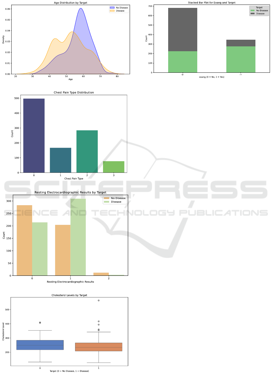
Figure 1(a) displays a distribution for age and

heart disease frequencies. The frequencies of the age

groups 50 - 60 years old and 60 - 70 years old are

relatively high, showing a pattern similar to a normal

distribution.

There are four forms of chest pain. From a

medical perspective, (i) is defined as substernal

discomfort brought on by emotional or physical stress

(Jones et al., 2020). A patient with typical angina has

a high risk of coronary artery blockages since their

past medical history exhibits the typical symptoms. (ii)

Chest pain that doesn't match the definition of typical

or classic chest pain is referred to as atypical

(Cleveland Clinic, 2023). (iii) The stabbing or knife-

like, protracted, dull, or uncomfortable condition that

can persist for brief or extended periods of time is

known as non-angina pain (Constant, 1990). ( ⅳ )

Asymptomatic pain does not manifest any signs of

illness or disease and may not be the source of or a

sign of a disease. The distribution of chest pain types

is as follows in Figure 1(b).

The rest distribution is as Figure 1(c) with three

resting electrocardiographic results 0, 1 and 2,

representing 3 different ranges. Cholesterol level can

be classified into two categories according to a target

value and can be inferred in Figure 1(d), while Exang

can be inferred in Figure 1(e).

Machine Learning Solutions for Heart Disease Diagnosis: Model Choices and Factor Analysis

(a)

(b)

(c)

(d)

(e)

Figure 1: Analysis of the important attributes. (a) is the Age

distribution by target, (b) is the Chest Pain type distribution,

is the Cholesterol Levels by target, (e) is the stacked bar

plot for Exang and Target. (Photo/Picture credit: Original).

3 MACHINE LEARNING IN

HEALTHCARE

Machine learning is a growing topic in recent

healthcare, which analyzes vast volumes of medical

data using algorithms. In the medical field, machine

learning algorithms are essential. Their pattern-

recognition capabilities in large datasets are well-

suited for genomics and proteomics applications.

They aid significantly in illness diagnosis and

detection, enabling better treatment decisions. As

medical data grows, the role of machine learning will

expand, promising more personalized and efficient

healthcare (Shailaja et al., 2018).

3.1 Explanation of Algorithms Used for

Diagnosis

Random forest, K-Nearest Neighbors (KNN),

Logistic Regression, Naive Bayes, Gradient Boosting

and Support Vector Machine (SVM) are evaluated for

heart disease diagnosis. Random forest is one

ensemble learning approach that exemplifies an

information mining methodology. It employs

multiple classifiers that work in tandem to identify the

class label for a new, unlabeled instance within a data

set (Parmar et al., 2019). A majority vote among the

individual decision trees determines the final forecast

for classification. Every tree makes a class prediction,

and the random forest predicts the class with the most

votes. Compared to a single decision tree, random

forests have the advantage of being able to handle

high-dimensional data well, being reasonably

ICDSE 2025 - The International Conference on Data Science and Engineering

resistant to overfitting, and being able to identify

intricate non-linear correlations in the data.

KNN is a learning algorithm that is instance-based.

When a new sample is provided, the KNN algorithm

locates the K samples in the training dataset that are

the most comparable (closest in distance) and then

uses the classes of these K neighbors to forecast the

new sample's class. Manhattan distance, Euclidean

distance, and other methods are typically used to

measure the distances between samples. It is

extensively utilized in domains including

recommendation systems, text categorization, and

image recognition. It is quite flexible with regard to

data distribution and does not require a training

procedure. One of its drawbacks is its high

computational complexity, which rises sharply with

data volume. Additionally, it is susceptible to local

noise in the data, and the model's performance may

be impacted by the K value selection.

Logistic regression is a linear model for

classification issues. It represents the likelihood that

a sample belongs to a particular class by mapping the

outcomes of linear regression to probability values

between 0 and 1. The likelihood function is

maximized in the model to estimate parameters, and

gradient descent is a popular solution technique. The

model can effectively handle linearly separable data

and is straightforward, interpretable, and

computationally efficient. Its restrictions on data

distribution, which typically call for feature

independence, are its drawbacks. Its capacity to fit

complex non-linear data is restricted, and it can only

handle linear relationships.

The Bayes theorem and the feature conditional

independence assumption form the foundation of the

Naive Bayes classification technique. It computes the

posterior probability of each class given the features

and makes the assumption that each feature is

independent given the class. The prediction outcome

is chosen from the class with the highest posterior

probability. This model is insensitive to missing

values, works well on small-scale data, and trains

quickly. The drawback is that the feature conditional

independence assumption is highly sensitive to the

input data's representation form and is frequently

challenging to meet in practice, which could

compromise the model's accuracy.

Based on the concept of ensemble learning,

gradient boosting trains a number of weak learners

iteratively before combining them to create a strong

learner. The approach gradually improves the

performance of the model by modifying the training

of the subsequent weak learner based on the gradient

of the current model's loss function in each iteration.

Numerous data kinds, including categorical and

numerical data, can be handled by it. It performs well

in generalization and has a strong fit for intricate non-

linear relationships. However, it is time-consuming to

train, prone to overfitting, and very sensitive to

hyperparameter selection, necessitating adjustment.

SVM maximizes the margin between the two

classes of samples by identifying the best hyperplane

to divide them. A kernel function is used to translate

the data to a high-dimensional space in order to make

it linearly separable in the high-dimensional space

while dealing with non-linear situations. SVM

performs well in handling both linear and non-linear

issues, has strong generalization ability, and

successfully prevents overfitting when working with

small sample data. The drawbacks include a lengthy

training period and considerable computational

complexity, particularly when working with huge

amounts of data. It also necessitates specific tuning

abilities and is highly sensitive to the kernel functions

and parameter choices.

4 MODEL TRAINING AND

COMPARISON

The six algorithms are properly applied in the process

of training and show different performances. To

evaluate the functionality of each algorithm, accuracy

and F1-score are calculated in Equation (1), and

Equation (2), using True Positive (TP), True Negative

(TN), False Positive (FP), False Negative (FN), with

P refers to precision and R refers to recall.

𝐴𝑐𝑐𝑢𝑟𝑎𝑐𝑦 =

TP + TN

TP + TN + FP + FN

(

)

𝐹1 =

2PR

P + R

(

)

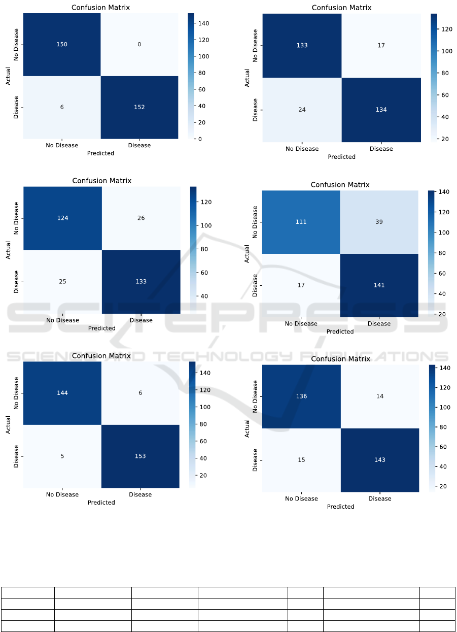
A key tool for assessing the effectiveness of

diagnostic tests, particularly in binary classification

settings, is the ROC curve (Srinivasan & Mishra,

2024), which is also used to compare various models.

A greater area under the curve typically indicates

higher performance. Figure 2 shows the inferred

confusion matrix reports, each of which represents an

algorithm. Table 2 lists the F1 Scores and Accuracy.

Figure 3 shows the ROC curve.

Machine Learning Solutions for Heart Disease Diagnosis: Model Choices and Factor Analysis

(a)

(b)

(c)

(d)

(e)

(f)

Figure 2: Confusion matrix for each model. (a) is the Random Forest confusion matrix, (b) is the Naive Bayes confusion

matrix, (c) is the Gradient Boosting confusion matrix, (d) is the KNN confusion matrix, (e) is the Logistic Regression

confusion matrix, (f) is the SVM confusion matrix. (Photo/Picture credit: Original).

Table 2: F1 score and accuracy.

Random Forest

Naive Bayes

Gradient Boosting

KNN

Logistic Regression

SVM

F1 for 0

0.98

0.83

0.96

0.87

0.80

0.90

F1 for 1

0.98

0.84

0.97

0.87

0.83

0.91

Accuracy

0.98

0.83

0.96

0.87

0.82

0.91

ICDSE 2025 - The International Conference on Data Science and Engineering

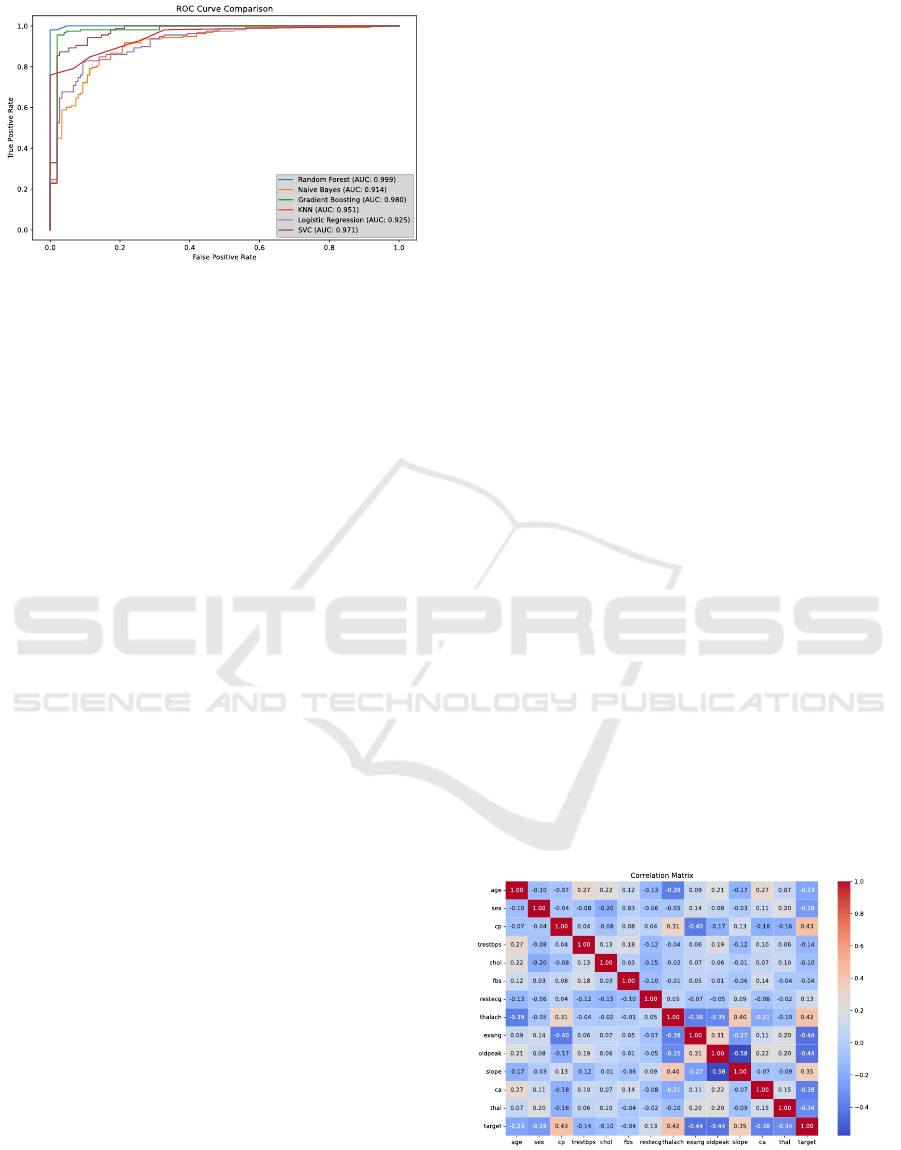
Figure 3: ROC curve for each model. (Photo/Picture credit:

Original).

Compared to other models, the Random Forest

classifier and Gradient Boosting performed better.

With the highest accuracy of 0.98, the Random Forest

classifier is closely followed by the Gradient

Boosting classifier, which has an accuracy of 0.96.

This suggests that in comparison to the other

classifiers, Random Forest and Gradient Boosting do

better overall at accurately classifying instances in

this data set. Random Forest has the highest precision

(0.96 & 1.00), whereas Gradient Boosting comes in

second (0.97 & 0.96). Gradient Boosting has a recall

of 0.96 and 0.97, both much higher than other models,

whereas Random Forest has a perfect recall of 1.00

for class 0 and 0.96 for class 1. With the greatest f1-

scores of 0.98 & 0.98 and 0.96 & 0.97, respectively,

Random Forest and Gradient Boosting demonstrate a

good trade-off between recall and precision. Figure 3

shows the ROC curves. Based on the Area Under

ROC Curve (AUC) values, the Random Forest model

performs the best, followed by Gradient Boosting and

SVM. In contrast, Naive Bayes, KNN, and Logistic

Regression are all above 0.900, indicating fairly high

functionalities, but they are all relatively weaker.

Random Forest or Gradient Boosting would be the

best options if overall high accuracy and strong

performance in both classes are the primary

objectives. These classifiers appear to be capable of

producing precise predictions and effectively

capturing the patterns in the data. Regarding feature

selection, Random Forest and Gradient Boosting

produced encouraging results when paired with the

computerized feature selection process (CFS) and the

medical knowledge-based motivated feature selection

process (MFS) (Nahar et al., 2013). This suggests that

it can improve its discriminatory power by efficiently

leveraging the improved feature sets.

Additionally, SVM does fairly well, with an

accuracy of 0.91. If Random Forest or Gradient

Boosting has too high of a computational cost, this

can be an acceptable substitute.

KNN performs mediocrely, with an accuracy of

0.87. It might work well with data sets when the local

similarity assumption is valid, but in this instance, the

best-performing classifiers exceed it.

The accuracy of Naive Bayes and Logistic

Regression is comparatively lower. The feature

independence assumed by Naive Bayes might not

hold true for this set of data. The intricacy of the

decision boundary in the data may be a limitation of

logistic regression. Despite its poorer performance,

logistic regression may still be taken into

consideration if interpretability and simplicity are

important since it can shed light on the link between

the target variable and the features.

5 RESULTS AND

INTERPRETATION

Using the six different methods of training, a

correlation matrix can be established in Figure 4. The

diagonal elements are all 1, indicating that each

variable is perfectly correlated with itself.

The correlation values are represented in the

matrix by a color gradient. A positive correlation is

shown in red and a negative correlation in blue.

Positive correlations imply that when one variable

rises, the other one tends to rise as well. When one

variable rises, the other one tends to fall, according to

negative correlations. For instance, there is a

somewhat negative association (-0.07) between age

and cp. Conversely, there is a moderately positive

connection (r = 0.22) between chol and trestbps.

Figure 4: Correlation Matrix. (Photo/Picture credit:

Original).

Machine Learning Solutions for Heart Disease Diagnosis: Model Choices and Factor Analysis

Table 3: significant correlations.

trestbps and chol

exang and oldpeak

age and exang

thalach and exang

0.22

0.40

-0.39

-0.38

Some significant correlations were included in

this correlation matrix and are shown in Table 3.

Trestbps is associated with higher chol and the same

as exang and oldpeak. Thalach and age are associated

with a lower likelihood of exang.

The feature cp has the highest importance value,

close to 0.25, while features like ca and thal also have

relatively high importance values, around 0.15. On

the other hand, features such as fbs, restecg, sex, and

exang have rather low importance values, with fbs,

nearly 0. Features with very low importance values

like fbs might be considered for removal if the goal is

to streamline the model.

6 CONCLUSIONS

Early diagnosis of heart disease plays a crucial role in

saving lives. Recognizing the significance of data

mining in facilitating heart disease diagnosis is of

utmost importance. This paper has elaborated on the

comparison of various classifiers for detecting heart

disease. It was noted that the Random Forest and

Gradient Boosting have emerged as a potentially

effective classification algorithm in this domain,

especially when total accuracy is regarded as the

performance metric. The results can also help in

feature selection, where less important features can be

removed to simplify the model without significantly

sacrificing accuracy. It also allows medical

practitioners to focus on the crucial aspects during

patient evaluations, potentially leading to earlier and

more accurate diagnoses.

There is an urgent need for further researches and

applications in this field to harness its full benefits

and continuously enhance the quality of healthcare,

ensuring more lives are saved and better health

outcomes are achieved.

REFERENCES

Ahsan, M. M., & Siddique, Z. 2022. Machine learning-

based heart disease diagnosis: A systematic literature

review. Artificial Intelligence in Medicine, 128, 102289.

Ahsan, M. M., Nazim, R., Siddique, Z., & Huebner, P. 2021.

Detection of COVID-19 patients from CT scan and

chest X-ray data using modified MobileNetV2 and

LIME. In Healthcare (Vol. 9, No. 9, p. 1099). MDPI.

Cleveland Clinic. 2023. Atypical chest pain. Retrieved from

https://my.clevelandclinic.org/health/symptoms/24935

-atypical-chest-pain

Constant, J. 1990. The diagnosis of nonanginal chest pain.

The Keio Journal of Medicine, 39(3), 187-192.

Jones, E., Johnson, B. D., Shaw, L. J., Bakir, M., Wei, J.,

Mehta, P. K., ... & Merz, C. N. B. 2020. Not typical

angina and mortality in women with obstructive

coronary artery disease: Results from the Women’s

Ischemic Syndrome Evaluation study (WISE). IJC

Heart & Vasculature, 27, 100502.

Nahar, J., Imam, T., Tickle, K. S., & Chen, Y. P. P. 2013.

Computational intelligence for heart disease diagnosis:

A medical knowledge driven approach. Expert Systems

with Applications, 40(1), 96-104.

Parmar, A., Katariya, R., & Patel, V. 2019. A review on

random forest: An ensemble classifier. In International

conference on intelligent data communication

technologies and internet of things (ICICI) 2018 (pp.

758-763). Springer International Publishing.

Shailaja, K., Seetharamulu, B., & Jabbar, M. A. 2018.

Machine learning in healthcare: A review. In 2018

Second international conference on electronics,

communication and aerospace technology (ICECA) (pp.

910-914). IEEE.

Stiglic, G., Kocbek, P., Fijacko, N., Zitnik, M., Verbert, K.,

& Cilar, L. 2020. Interpretability of machine learning-

based prediction models in healthcare. Wiley

Interdisciplinary Reviews-Data Mining and Knowledge

Discovery, 10(5).

Srinivasan, A., & Mishra, A. 2024. Receiver Operating

Characteristic (ROC) Curve Analysis for Diagnostic

Studies. In R for Basic Biostatistics in Medical

Research (pp. 253-258). Springer, Singapore.

World Health Organization. 2021. Cardiovascular disease.

Retrieved from https://www.who.int/health-

topics/cardiovascular-diseases#tab=tab_1

ICDSE 2025 - The International Conference on Data Science and Engineering