Sheet Metal Forming Springback Prediction Using Image Geometrics

(SPIG): A Novel Approach Using Heatmaps and Convolutional Neural

Network

Du Chen

, Mariluz Penalva Oscoz

, Yang Hai

, Martin Rebe Ander

, Frans Coenen

and Anh Nguyen

Department of Computer Science, The University of Liverpool, Liverpool, L693BX, U.K.

TECNALIA, Basque Research and Technology Alliance, Sebastian, Spain

Nanjing EITRI, Nanjing, China

Keywords:

Single Point Incremental Forming, Springback Prediction, Image Geometries, Deep Learning, Convolutional

Neural Network.

Abstract:

We propose the Springback Prediction Using Image Geometrics (SPIG) approach to predict springback errors

in Single Point Incremental Forming (SPIF). We achieved highly accurate predictions by converting local

geometric information into heatmaps and employing ResNet based method. Augmenting the dataset twenty-

four-fold through various transformations, our ResNet model signiﬁcantly outperformed LSTM, SVM, and

GRU alternatives in terms of the MSE and RMSE values obtained. The best performance result in an R²

value of 0.9688, 4.95% improvement over alternative methods. The research demonstrates the potential of

ResNet models in predicting springback errors, offering advancements over alternative methods. Future work

will focus on further optimisation, advanced data augmentation, and applying the method to other forming

processes. Our code and models are available at https://github.com/DarrenChen0923/SPIF.

1 INTRODUCTION

Single Point Incremental Forming (SPIF)(Martins

et al., 2008) is an advanced sheet metal cold form-

ing technique that uses a Computer Numerical Con-

trol (CNC) machine to manufactured desired shapes.

The alternative is hot forming where the material to

be fabricated is ﬁrst heated up. Cold forming does

not require this. Therefore, cold forming is more cost-

effective and eco-friendly than hot forming. The dis-

advantage of SPIF cold forming is that the process

features springback, a property of metals where the

material tries to return to its original shape after bend-

ing. This means that the manufactured shape is differ-

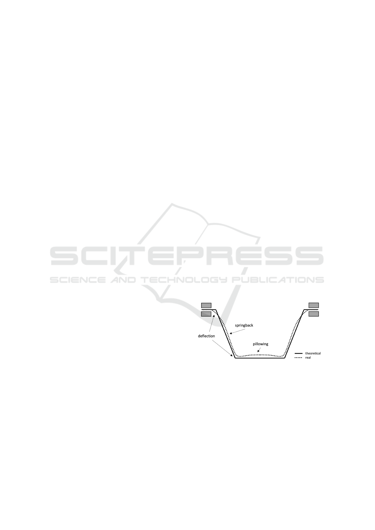
ent from the speciﬁed shape CAD. This is illustrated

in the Figure 1, which shows a ﬂat-topped pyramid

shape. The solid line is the pre-speciﬁed CAD shape,

while the dashed line is the ﬁnal shape. An inspection

of the ﬁgure shows that the two shapes are not the

same. Therefore Springback errors can cause devia-

tions between the ﬁnal formed part and the intended

shape, which is particularly important in ﬁelds such as

aerospace manufacturing where extremely high part

accuracy is required. Geometric accuracy in the SPIF

process remains a major challenge due to the spring-

back effect.

Figure 1: Illustration of the springback effect when con-

ducting cold sheet metal forming.

Path correction and springback error prediction

methods have evolved with the advent of artiﬁ-

cial intelligence, particularly deep learning, enhanc-

ing accuracy. For example, Artiﬁcial Neural Net-

works (ANNs), regression, and other AI techniques

have all been considered effective solutions (Bahloul

et al., 2013; Spathopoulos and Stavroulakis, 2020;

Zwierzycki et al., 2017). The challenge is how to de-

ﬁne the training data required for various AI learn-

ers to effectively represent local geometries so that

Chen, D., Oscoz, M. P., Hai, Y., Ander, M. R., Coenen, F. and Nguyen, A.

Sheet Metal Forming Springback Prediction Using Image Geometrics (SPIG): A Novel Approach Using Heatmaps and Convolutional Neural Network.

DOI: 10.5220/0013673100004000

Paper published under CC license (CC BY-NC-ND 4.0)

In Proceedings of the 17th International Joint Conference on Knowledge Discovery, Knowledge Engineering and Knowledge Management (IC3K 2025) - Volume 1: KDIR, pages 28-38

the springback of previously unseen parts can be pre-

dicted. Muhamad et al.(Khan et al., 2015), writing

in 2015, propose a strategy to represent local geom-

etry as a series of points. The goal is to create a set

of local geometries that are a superset of all possible

local geometries of any part we may wish to manu-

facture. The work introduced in (Khan et al., 2015)

used k-Nearest Neighbour (kNN) classiﬁcation, a ma-

ture machine learning classiﬁcation technique, and

proved that the proposed method worked well. Du

Chen et al. (Chen et al., 2023) proposed a method

based on GRU (Gated Recurrent Unit) and data aug-

mentation technology that signiﬁcantly expanded the

dataset size through data augmentation and used the

GRU model to predict springback error, achieving ex-

cellent results. Their research showed that by repre-

senting local geometry as a point sequence and com-

bining it with deep learning, the accuracy of spring-

back error prediction can be effectively improved.

However, the above methods have shortcomings

when expressing local geometric information and

processing complex geometric relationships, limiting

further improvement in prediction accuracy. The Lo-

cal Geometry Matrix (LGM) and Local Distance Met-

ric (LDM) methods proposed in (El-Salhi et al., 2012;

El-Salhi et al., 2013), although they have improved

the accuracy of geometric representation to a certain

extent, still had limitations in processing complex ge-

ometric shapes. Moreover, existing methods mostly

used LSTM models. Although they perform well

in processing sequence data, their structure entails a

computational overhead.

Building on previous research, we propose the

springback prediction using the Image Geometrics

(SPlF) approach to springback prediction. An ap-

proach that features three novel elements: ﬁrstly

a new local geometry expression method using

heatmaps to capture the geometric information of lo-

cal areas. A method that can more intuitively and ac-

curately represent local geometric features. Second,

we convert the local geometry problem into an image

processing problem and use a few residual blocks to

process heatmaps, improving prediction accuracy and

robustness. Thirdly the use of a ResNet Model. Ex-

periments demonstrated the superior performance of

the ResNet model in springback error prediction, sig-

niﬁcantly better than all previous methods. The exper-

imental results reported later in this paper show that

this new method achieves better results, with a best

R2 value of 0.9688 compared to the previous best R2

value of 0.9228 (Chen et al., 2023), an increase of

4.95%.

To summarize the above, our contributions are as

follows:

1. The use of heatmaps to capture local geometric

details accurately.

2. Converting the local geometry problem into an

image-processing task for better prediction.

3. Demonstrating ResNet’s superior performance

over previous methods in springback prediction.

The rest of this paper is organized as follows:

Section 2 presents the related work underpinning the

work presented. Section 3 introduces the method

in detail, including presenting the proposed SPIG

approach, problem transformation, and the ResNet

model. The experimental design and results are pre-

sented and discussed in Section 4. The paper is con-

cluded in Section 5 with a summary of the main con-

tributions of this paper and proposes future research

directions.

2 RELATED WORK

In the SPIF process, predicting springback error has

been a signiﬁcant research direction. Various regres-

sion methods have been employed to model and pre-

dict these errors. For instance, multiple linear re-

gression (Tranmer and Elliot, 2008), regression trees

(Loh, 2011), Support Vector Machines (SVM) (Boser

et al., 1992), and Gaussian processes (Seeger, 2004)

are common approaches (Bahloul et al., 2013). Ad-

ditionally, genetic algorithms (Holland, 1975) com-

bined with ﬁnite element simulations (Belytschko and

Hodge Jr, 1970) have been used to optimize mould-

ing parameters and reduce springback error (Maji and

Kumar, 2020). However, these traditional methods

often struggle with complex geometric relationships.

Deep learning has recently been applied to spring-

back error prediction. For instance, a GRU-based

method combined with data augmentation signiﬁ-

cantly expanded the dataset and achieved excellent

results (Chen et al., 2023). The LSTM model cap-

tures time correlations of springback errors, improv-

ing prediction accuracy (Bingqian et al., 2024). Other

studies have integrated ﬁnite element simulation with

machine learning to optimize forming parameters and

sheet shapes, thus reducing springback (Sbayti et al.,

2020; Spathopoulos and Stavroulakis, 2020). No-

tably, combining ﬁnite element simulation with neu-

ral network-based optimization has proven effective

(Spathopoulos and Stavroulakis, 2020).

Representing local geometric information is cru-

cial in springback error prediction. Traditional meth-

ods often rely on point sequences (El-Salhi et al.,

2012), while the local geometry matrix (LGM) and

local distance metric (LDM) methods use grids to rep-

Sheet Metal Forming Springback Prediction Using Image Geometrics (SPIG): A Novel Approach Using Heatmaps and Convolutional

Neural Network

resent geometric shapes (El-Salhi et al., 2012; El-

Salhi et al., 2013). Point sequence methods typi-

cally employ k-nearest neighbour (kNN) (Fix, 1985)

and dynamic time warping (DTW) (Sakoe and Chiba,

2003) for classiﬁcation (Khan et al., 2012; Khan et al.,

2015). Despite improvements in geometric represen-

tation accuracy, these methods struggle with complex

geometric changes, limiting their predictive accuracy.

Recent approaches have integrated sophisticated tech-

niques like machine learning and ﬁnite element simu-

lations to enhance prediction accuracy, aiming to cap-

ture more intricate geometric details and complex re-

lationships in forming processes.

Image processing techniques, especially convolu-

tional neural networks (CNN) (LeCun et al., 2002),

excel at capturing complex geometric relationships.

CNNs automatically extract features from images

and perform efﬁcient learning through deep network

structures. Other notable techniques include edge de-

tection methods like the Canny edge detector (Canny,

2009), the Scale-Invariant Feature Transform (SIFT)

(Lowe, 2004), and the Hough transform (Duda and

Hart, 1972) for detecting shapes. Morphological im-

age processing techniques (Serra, 1983), such as di-

lation and erosion, provide support for shape analysis

and noise removal. The Harris corner detector (Har-

ris et al., 1988) identiﬁes key points in images. Gen-

erative models like Generative Adversarial Networks

(GANs) (Goodfellow et al., 2014) and Variational Au-

toencoders (VAEs) (Kingma et al., 2013) have been

used for data augmentation by adding realistic noise,

enhancing training datasets and improving model ro-

bustness.

Integrating recent high-quality studies contextu-

alizes our contributions within the broader land-

scape of springback prediction research. For in-

stance, a Simulated Annealing Particle Swarm Opti-

mization (SAPSO) optimized Support Vector Regres-

sion (SVR) algorithm has been proposed for high-

accuracy springback prediction, demonstrating the

application of machine learning in bending processes

(He et al., 2025). A springback prediction model

for DP780 steel using a modiﬁed Yoshida-Uemori

two-surface hardening model has been shown to sig-

niﬁcantly enhances prediction accuracy (Zajkani and

Hajbarati, 2017). Optimized constitutive equations

in TRIP1180 steel cold stamping also show sub-

stantial improvements in prediction accuracy (Seo

et al., 2017). Additionally, a springback prediction

model for multi-cycle bending, validated through ex-

tensive experimental data, has been developed based

on different hardening models (Zajkani and Hajbarati,

2017). An anisotropic hardening model for high-

strength steel has also been introduced, demonstrat-

ing effectiveness in both numerical and experimental

studies (Zeng and Xia, 2005). These studies highlight

the importance of advanced optimization algorithms

and reﬁned material models in enhancing springback

prediction accuracy.

In our research, we convert local geometric infor-

mation into heatmaps and utilize the ResNet model

for processing (He et al., 2016). This approach sig-

niﬁcantly improves springback error prediction, out-

performing previous methods. Leveraging CNNs for

detailed geometric information provides robust and

accurate predictions. Transforming the problem into

an image-processing task enhances feature extraction

capabilities, leading to superior accuracy and stabil-

ity. Additionally, data augmentation techniques like

rotation, ﬂipping, scaling, and translation expand the

dataset, further improving model robustness.

3 METHODOLOGY

3.1 The Springback Prediction Using

the Image Geometries (SPIG)

The core component of the proposed Springback Pre-

diction using Image Geometries (SPIG) approach is

generating the required local geometry images. The

proposed process is discussed in Sub-section 3.1.2.

The resulting image set D = {I

,...} is then the

input to a prediction model to produce springback

predictions for the item to be manufactured, which

can then be applied in reverse to the CAD deﬁnition

to produce a corrected deﬁnition. The calculation of

springback error values corresponding to the images

is described in Sub-section 3.1.1.

Algorithm 1 presents the overall process of sprin-

back error calculation. To accommodate multiple

scales of local features with different grid sizes, the

entire heatmap is divided into w × w sub-images,

where w/3 can be 5mm, 10mm, 15mm, or 20mm.

Therefore, the sub-images sizes become 15 × 15 mm,

30 × 30 mm, 45 × 45 mm, and 60 × 60 mm, respec-

tively. Changing these grid sizes allows the algorithm

to capture local geometry, intensity distribution, or

other relevant properties at different resolution levels.

3.1.1 Springback Error Calculation

The springback calculation Algorithm 1, computes

the springback error for each point in the input grid

set by measuring the distance between each input grid

point and its corresponding point in the output grid

set, as outlined in (El-Salhi et al., 2012; Gill et al.,

2021; Salomon, 2006). The algorithm takes two sets

KDIR 2025 - 17th International Conference on Knowledge Discovery and Information Retrieval

Algorithm 1: Calculate Springback Error.

Input: G

(input grid), G

out

(output grid)

Output: E (set of springback errors)

E ← {};

for each g

in G

plane g

← FitPlane(g

);

intersect point ← FindIntersection(g

out

);

if intersect point found then

← Distance(g

,intersect point);

E ← E ∪ {s

};

else

E ← E ∪ {0};

return E;

Function FitPlane(g,G):

Fit a plane to the grid point g and its

neighbours in grid G plane

return plane

Function FindIntersection(g

out

for each g

in G

out

plane g

← FitPlane(g

out

)

intersect point ←

CalculateIntersection(g

, planeg

)

if intersect point found then

return intersect point

return null

Function

CalculateIntersection(point, plane):

Calculate the intersection point of a normal

from point with the plane intersect point

return intersect point

Function Distance(point

, point

Calculate the Euclidean distance between two

points distance

return distance

of grid points, G

(input grid points) and G

out

(out-

put grid points), and produces a set E containing the

springback errors.

The algorithm initializes an empty error set E to

store the calculated errors for each grid point. It it-

erates through each grid point g

in the input grid

. For each point, it ﬁts a plane to g

and its

neighbouring points in G

using the FitPlane func-

tion to establish a local reference plane. The algo-

rithm then determines the intersection point of the

normal from g

with the plane deﬁned by G

out

us-

ing the FindIntersection function. If an intersec-

tion point is found, it calculates the distance s

be-

tween the intersection point and g

using the Distance

function. This distance, representing the springback

error for that grid point, is added to E. If no in-

tersection point is found, a value of 0 is added to

E. Finally, the algorithm returns the set E, contain-

ing the springback errors for all input grid points,

providing a comprehensive measure of deviations

across the entire grid. Several helper functions have

been included to ensure efﬁciency and accuracy:

FitPlane, FindIntersection, CalculateIntersection,

and Distance. FitPlane ﬁts a plane to a grid point

and its neighbours; FindIntersection ﬁnds the inter-

section of a normal with G

out

’s plane; and Distance

calculates the Euclidean distance between two points.

In summary, the springback calculation algorithm

accurately computes the springback error for each in-

put grid point, generating a set of errors that can be

used to train a springback prediction model.

3.1.2 Local Geometry Image Generation

As noted in the introduction to this section, using

images to represent local geometry is central to the

proposed SPIG approach. The choice of heatmaps

as a representation for local geometric information

is driven by their ability to encode spatial relation-

ships effectively. Convolutional Neural Networks

(CNNs) can then be used to extract hierarchical spa-

tial features. This approach avoids the need for exten-

sive feature engineering and naturally integrates with

ResNet’s architecture, enhancing both accuracy and

computational efﬁciency. Additionally, the heatmap

format facilitates advanced data augmentation tech-

niques, such as rotation and ﬂipping, which improve

model robustness and generalization.

The process of extract sub-images involves two

key steps. First, a heatmap H is generated with ref-

erence values corresponding to the z values in the F

point cloud. This heatmap visualizes the surface char-

acteristics and variations of the input data by mapping

the z values to colour intensities, creating a detailed

and intuitive representation of local geometrical fea-

tures. Next, a set of sub-images is extracted from the

heatmap H using a sliding window technique with a

predeﬁned window size w. This method systemat-

ically captures various portions of the heatmap, re-

sulting in a comprehensive set of local geometry im-

ages D = {I

,...}. Each sub-image encapsulates

speciﬁc local geometrical details, allowing the model

to analyze and predict springback errors with greater

precision. By focusing on localized sections of the

heatmap, the SPIG approach ensures that subtle vari-

ations in geometry are accounted for, enhancing the

model’s accuracy and robustness.

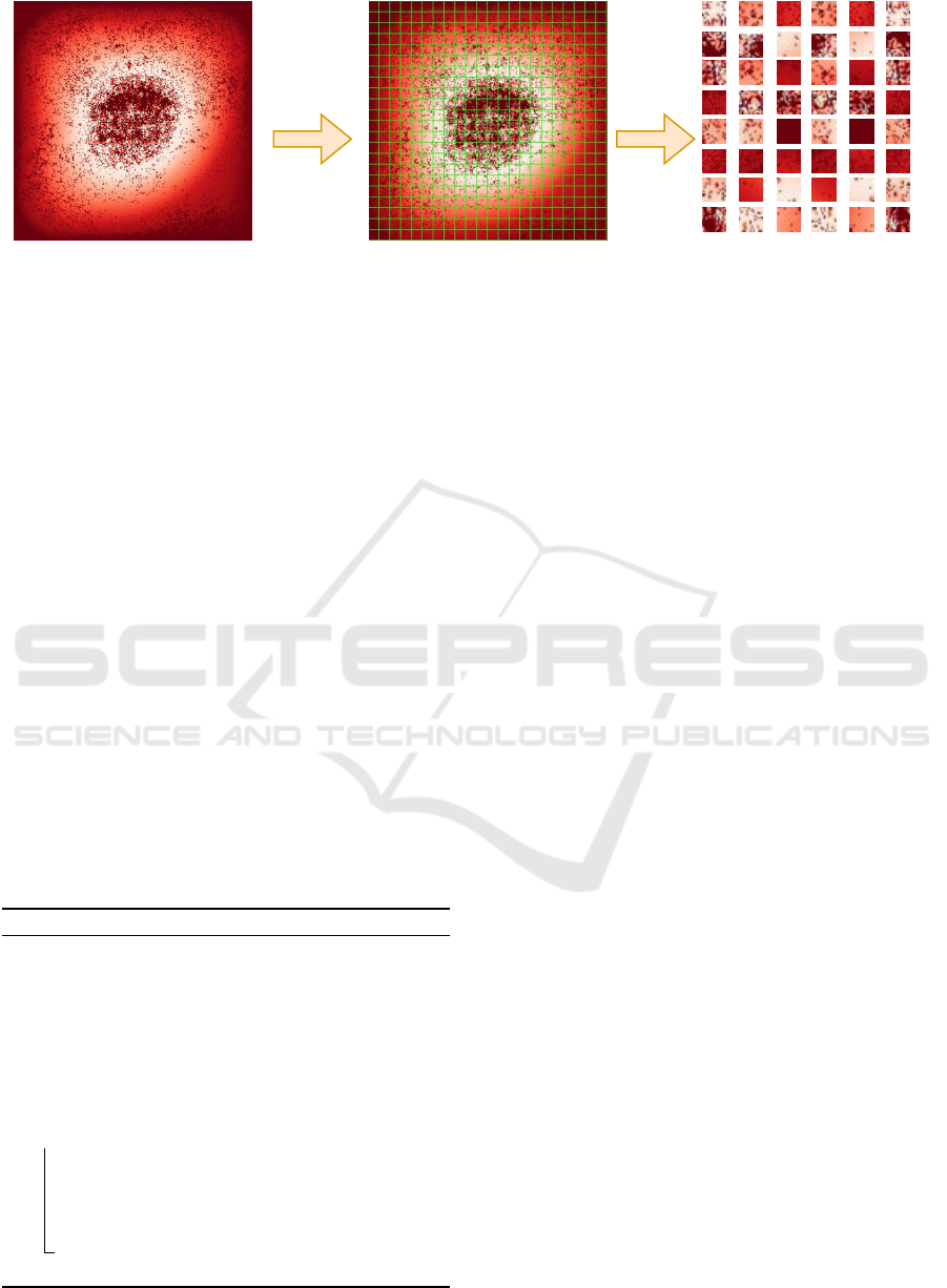
Figure 2 illustrates the heatmap generation and

processing for springback error prediction. Figure 2

features a heatmap, generated from a ﬂat-topped pyra-

mid shape that uses a white-to-red colour gradient to

represent z values, with white indicating smaller val-

ues and red indicating larger values. The raw heatmap

H shows the z values of the pyramid shape. This

heatmap is then divided into w ×w sub-images, which

serve as inputs for the springback prediction model,

Sheet Metal Forming Springback Prediction Using Image Geometrics (SPIG): A Novel Approach Using Heatmaps and Convolutional

Neural Network

Cropping

by w*w

(a) Raw Heatmap H showing the z

values of the flat-topped pyramid shape

(b) Heatmap H divided into w*w

sub-images for input inot the prediction model

examples from the sub-image dataset

Figure 2: Example of a heatmap: (a) Raw heatmap H illustrating z values using a red-to-white scale; (b) Heatmap H divided

into w × w sub-images for springback prediction input.

capturing local geometric features. Randomly sam-

pled sub-images from the dataset were used for model

training and validation, highlighting the importance

of each step in accurately predicting springback er-

rors.

3.1.3 Training Set Generation

The springback calculation algorithm is designed to

compute the springback error for each point in the in-

put grid set. Springback error is determined by mea-

suring the distance between each input grid point and

its corresponding point in the output grid set. Us-

ing the method outlined in (El-Salhi et al., 2012; Gill

et al., 2021; Salomon, 2006), one can determine the

error assuming that a grid square g

belongs to G

and

a matched grid square g

belongs to G

out

. The algo-

rithm, Algorithm 1, takes as input two sets of grid

points, G

(the input grid points) and G

out

(the out-

put grid points), and produces a set E containing the

springback errors for each point.

Algorithm 2: Training Set Generation.

Input: F

, F

out

, and w

Output: T (training set)

T ← ∅;

H ← Heatmap generated from F

; // See

Sub-section 3.1.2

← Input grid generated from F

using grid

size w/3;

out

← Output grid generated from F

out

using grid

size w/3;

foreach g

in G

← Calculated springback value ; // See

Sub-section 3.1.1

← Sub-image from H for grid square g

;

// See Sub-section 3.1.2

T ← T ∪ ⟨I

⟩;

return T ;

This pseudocode (Algorithm 2) outlines the pro-

cedure for generating a training set T used in a model

that predicts springback (or some other desired out-

put) from given input ﬁelds F

and F

out

. The al-

gorithm starts by initializing an empty training set

T . Then, a heatmap H is generated from F

; this

heatmap often encodes spatial or intensity-related in-

formation that will be used as part of the input fea-

tures.

Next, two grids are created: G

from F

and G

out

from F

out

. Both grids use a particular granularity or

cell size (w/3 in this example), dividing the input and

output images (or ﬁelds) into smaller squares or seg-

ments. These smaller grid squares serve as the basis

for localized analysis and feature extraction.

The algorithm then iterates over each grid cell g

in G

. For every cell, it calculates a corresponding

springback value s

, presumably by comparing the lo-

cal geometry or other relevant parameters between F

and G

out

. This step references a sub-section in the text

3.1.1 that presumably contains more details on how

the springback value is derived.

Simultaneously, a sub-image I

is extracted from

the heatmap H for the region deﬁned by g

. This sub-

image, corresponding to the same local region as g

contains the relevant features needed for training the

model—such as local curvature, gradient, intensity,

or temperature distributions, depending on the appli-

cation. The method for extracting or computing this

sub-image is detailed in another sub-section 3.1.2.

Finally, the pair (I

) is added to the training set

T . By collecting these pairs across all grid cells,

the algorithm assembles a comprehensive training set

that maps localized input features (sub-images of H)

to corresponding output labels (the computed spring-

back values). At the end, the completed training set T

is returned for subsequent model training or analysis.

KDIR 2025 - 17th International Conference on Knowledge Discovery and Information Retrieval

3.2 Problem Transformation

In traditional springback error prediction methods, lo-

cal geometric information is typically represented by

point sequences or local geometric matrices. These

methods have limitations when dealing with complex

geometries and nonlinear deformations. To address

these issues, we propose converting the springback

error prediction problem from a geometric problem

to an image processing problem.

Traditional methods often require manual feature

design and struggle to fully capture geometric details.

In contrast, Convolutional Neural Networks (CNNs)

excel at processing high-dimensional and complex-

structured data, automatically extracting multi-level

features from images. This makes CNNs ideal for

processing geometric data represented by heatmaps.

The detailed steps for generating heatmaps were ex-

plained in Section 3.1.

To adapt to the input requirements of CNNs,

we performed several preprocessing steps on the

heatmaps. First, all heatmaps were resized to 342 ×

342 pixels to ensure uniform dimensions. This re-

sizing step was essential for maintaining consistency

in the data fed into the CNN, allowing the model to

process the images efﬁciently without discrepancies

caused by varying image sizes. Next, we cropped

the heatmaps according to different grid sizes (5, 10,

15, and 20), maintaining a 3 × 3 structure for the

sub-images. For instance, with a grid size of 10,

the heatmap would be divided into multiple 30 × 30

blocks. This method of cropping and resizing ensures

that the input images are standardized in size and seg-

mented to highlight relevant local geometrical varia-

tions, thereby enhancing the model’s ability to accu-

rately predict springback errors.

To increase the diversity of training data and im-

prove the generalization ability of the model, we

adopted various data augmentation techniques, in-

cluding rotation, ﬂipping, scaling, and translation.

These data augmentation techniques generate more

training samples, improving the prediction accuracy

of the model in different scenarios. The preprocessed

and augmented heatmaps were used as input for the

CNN. ResNet extracts multi-level features through

multiple convolution and pooling layers, and the fully

connected layer outputs the predicted springback er-

ror. This approach leverages CNN’s strengths in fea-

ture extraction, leading to more accurate and robust

predictions.

3.3 Heatmap-Based Neural Framework

for Springback Prediction (HNFSP)

The prediction model employed was ResNet (Resid-

ual Network) (LeCun et al., 2002). ResNet is a

deep convolutional neural network. By introducing

a residual structure, it effectively solves the gradient

vanishing and gradient exploding problems in deep

networks. This feature enables ResNet to maintain

efﬁcient training capabilities as the network depth

increases and is particularly suitable for processing

high-dimensional image data with complex geometric

features. Compared with traditional time series mod-

els (such as LSTM and GRU), ResNet has signiﬁcant

advantages in processing spatial information (such as

geometric changes and local feature capture).

A range of values w/3 was considered from 5mm

to 20mm, increasing in steps of 5mm, to determine

the most appropriate image/grid size for optimal per-

formance. The advanced ResNet model consisted of

N Residual blocks; N was set to 3 when the grid

size was 5 mm and to 4 when the grid size was 10,

15, and 20mm. Each residual block was composed

of two 3 × 3 convolutional layers for feature extrac-

tion and one dense (fully connected) layer with a sin-

gle node for predicting springback error. An average

pooling layer was included after the residual blocks

to reduce spatial dimensions while retaining essential

features, and the ﬁnal springback error prediction is

output through the fully connected layer. The resid-

ual block introduces skip connections, which enables

the network to effectively transmit input information

and allows gradients to be directly passed back to

the previous layers. This not only reduces the difﬁ-

culty of training deep networks but also enables the

model to capture richer local features (such as geo-

metric changes) and global features (such as overall

shape changes). This feature is particularly impor-

tant in the springback prediction problem because the

local deformation and global springback characteris-

tics of metal sheets are usually intertwined in a multi-

scale manner.

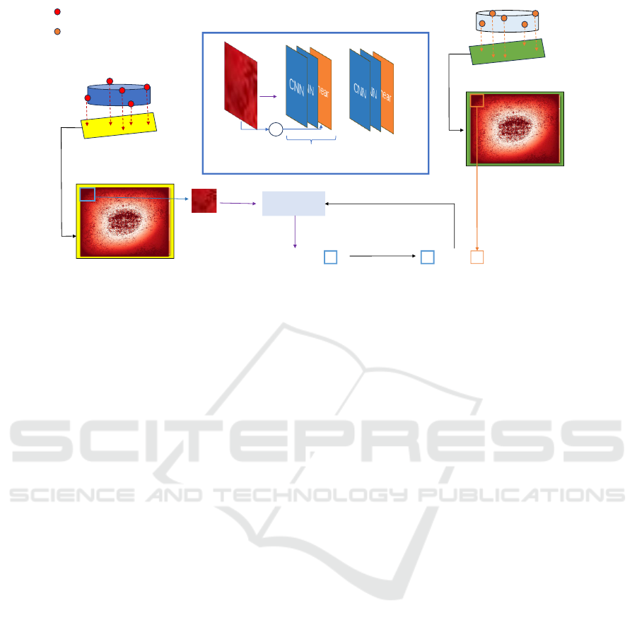
Additionally, a feature fusion layer and a regres-

sion output layer were added in the custom module

to better address the speciﬁc task of springback error

prediction. The detailed architecture is illustrated in

Figure 3. For comparison, the same shape used in the

ResNet model was employed to generate a time series

representation, as discussed in Section 2. This repre-

sentation was used to construct three additional pre-

diction models to be used for comparison purposes:

LSTM, SVM and GRU.

The main process of the ResNet model included

several steps: generating heatmaps from the point

Sheet Metal Forming Springback Prediction Using Image Geometrics (SPIG): A Novel Approach Using Heatmaps and Convolutional

Neural Network

Expected Raw Pointcould Points

0.2 0.4 0.3 0.4 0.4 0.5

0.6 0.4 0.4 0.2 0.4 0.3

0.2 0.4 0.3 0.2 0.4 0.3

Z value

Heatmap

ResNet

Predicted Error of Area

Expected Raw

Pointclouds

Expected 2D Vector

v.s.

Real Raw Pointcould Points

Z value

Ground Truth Raw

Pointclouds

0.2 0.4 0.3 0.4 0.4 0.5

0.6 0.4 0.4 0.2 0.4 0.3

0.2 0.4 0.3 0.2 0.4 0.3

Real 2D Vector

Ground Truth Error

MSE Loss

Residual Block

….

Heatmap ResNet

Figure 3: Heatmap-Based Neural Framework for Springback Prediction (HNFSP).

cloud and cropping the heatmaps according to the

speciﬁed grid size to obtain a sub-image dataset and

input it into the ResNet model. Features were ex-

tracted through multiple residual blocks, and the pre-

dicted springback error generated through a fully con-

nected regression layer. The Mean Squared Error

(MSE) loss function was used to calculate and com-

pare the predicted error with the expected error, pro-

viding a measure of model performance and enabling

comparison with the time series-based models. This

approach was forward to improve prediction accu-

racy. It was conjectured that this was because the

spatial structure of heatmap data was a natural match

for the convolution operation of ResNet. The fea-

tures extracted by the convolution layer could not only

capture the local deformation reﬂected by the differ-

ent color gradients in the heatmap, but could also

gradually capture more advanced geometric features

through multi-level convolution. For example, at a

larger grid size, ResNet could more effectively cap-

ture the overall deformation trend; at a smaller grid

size, its residual block can focus on the changes in

local geometric details.

Compared with the time series models (LSTM,

GRU), the convolution operation of ResNet could efﬁ-

ciently process two-dimensional heatmap data and di-

rectly extract spatial features without designing com-

plex sequence input methods. In addition, compared

with traditional SVM methods, ResNet can better

handle nonlinear and high-dimensional data, so it per-

formed better in predicting complex geometric defor-

mations (such as springback error).

4 EXPERIMENT

4.1 Experiment Settings

For the evaluation, a titanium alloy (Ti-6Al-4V) ﬂat-

topped pyramid shape (342 × 342×30mm) was used,

which is the standard shape for evaluating springback

prediction, similar to the shapes used in (Chen et al.,

2023; El-Salhi et al., 2012; El-Salhi et al., 2013; Khan

et al., 2012; Khan et al., 2015). For the proposed

SPIG approach, the dataset was augmented by: (i) ro-

tating each image through 90, 180, and 270 degrees;

(ii) ﬂipping the original image; and (iii) rotating the

ﬂipped image through 90, 180, and 270 degrees, re-

sulting in a seven-fold increase in training data size.

The experimental steps include data preprocess-

ing, model training, and validation. First, we col-

lected CAD (G

) and actual (G

out

) point cloud data

and converted them into 342 × 342 heatmaps, then

standardized and enhanced them. The dataset was

split into training and validation sets in an 8:2 ratio.

We applied data augmentation techniques such as ro-

tation, ﬂipping, scaling, and translation to increase

data diversity. The batch size was 64, with 1000

epochs and a learning rate of α = 0.0001. We used

the Adam optimization algorithm with mean square

error (MSE) as the loss function. The preprocessed

data were then used to train the ResNet model, with

appropriate parameters set and continuous monitoring

of loss value and evaluation metrics.

Finally, the model’s prediction performance was

evaluated using the validation set, and the evaluation

indicators recorded and analyzed to compare the per-

KDIR 2025 - 17th International Conference on Knowledge Discovery and Information Retrieval

formance differences under different models and set-

tings. Model performance was assessed using Mean

Absolute Error (MAE), Mean Square Error (MSE),

Root Mean Square Error (RMSE), and determination

coefﬁcient values (R²).

The rest of this section is organised as follows:

The point series local geometry representation, with

which the proposed SPIG approach was compared,

is considered in further detail in section 4.2. The

two evaluation objectives are then considered in Sub-

sections 4.4 and 4.5 respectively.

4.2 Point Series Approach

The operation of the proposed SPIG approach

was compared with three-point series-based models,

LSTM, SVM, and GRU. Details concerning these

models were presented previously in (Chen et al.,

2023). However, for completeness, a brief description

of the process for generating local geometry point se-

ries representations is presented here.

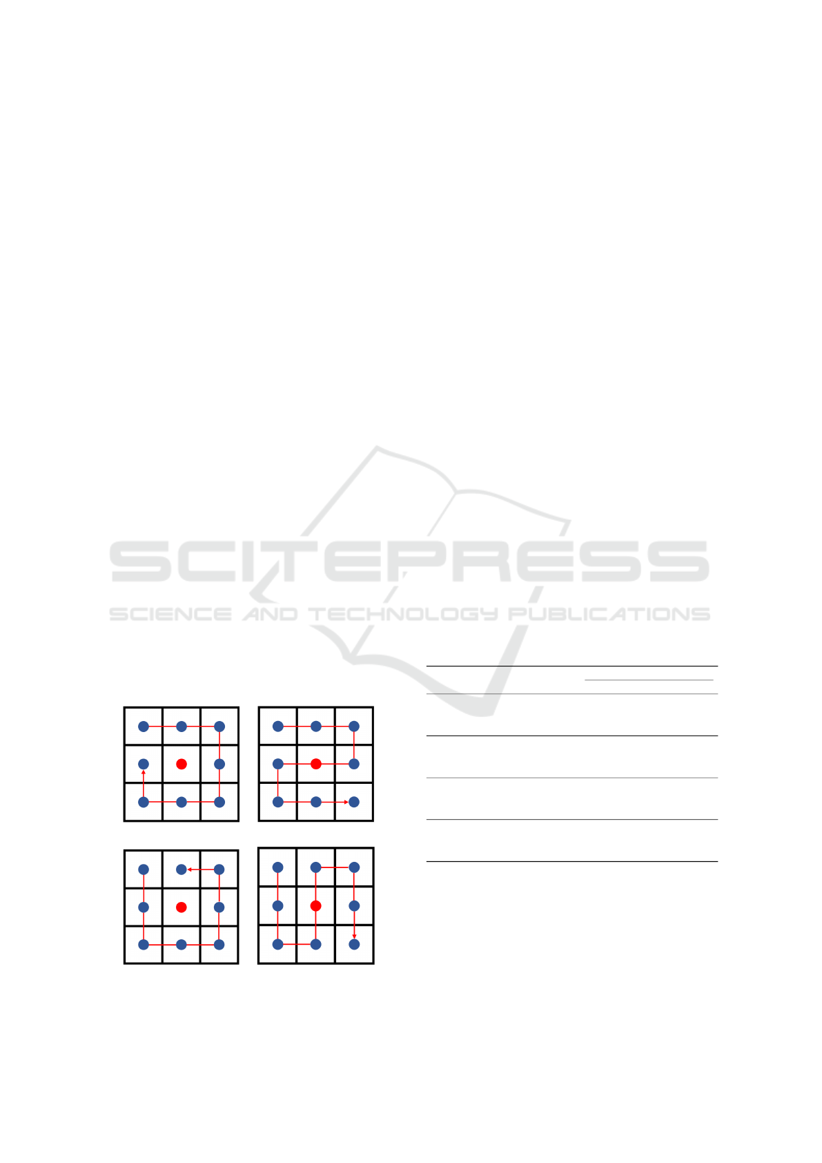
As seen in Figure 4, the goal is to represent the

local geometry around each g

∈ G

in terms of the

z value difference between g

and each of its neigh-

bouring grid squares. A labelled point series P =

⟨P,e⟩ = ⟨[p

, p

,..., p

],e⟩ was used to represent each

∈ G

. Here, e is the associated springback value

in E, and p

is the difference in z values between

grid square g

and its neighbour g

. Many conﬁgura-

tions exist for these point series, but the most straight-

forward is to look at each grid square in G

’s eight

immediate neighbours (three at corners and ﬁve at

edges), as illustrated in Figure 4. As long as the point

series are formed consistently, the order in which they

are generated is irrelevant.

(a) Clockwise. (b) Z-Sequence.

Figure 4: Example of point series generation.

After calculating the set of errors {e

,...} and

the set of point series {P

,...}, the errors and

point series can be added to the training set D

train

,...}, where each T

= ⟨P

⟩.

4.3 Experiment Result

The evaluation results are presented in Table 1. From

the table it can be seen that the ResNet model per-

forms better than LSTM, GRU, and SVM models

with respect to all metrics (MAE, MSE, RMSE, and

R2) for all grid sizes (5mm, 10mm, 15mm, and

20mm). ResNet provides the greatest beneﬁt at big-

ger grid sizes, and prediction accuracy typically in-

creases with grid size. For instance, ResNet out-

performs GRU (0.2566), LSTM (0.3067), and SVM

(0.4569) with an MAE of 0.1909 at a 5mm grid size.

ResNet has a mean square error (MSE) of 0.0258,

whereas GRU, LSTM, and SVM have MSEs of

0.1747, 0.1640, and 0.1452, respectively, with a grid

size of 20 mm. Furthermore, ResNet continuously ob-

tains the greatest R2 values (e.g., 0.9688 at 10 mm),

demonstrating its better neural design for capturing

spatial data.whereas SVM is computationally efﬁ-

cient, it suffers from the nonlinear, high-dimensional

nature of spatial feature extraction, whereas LSTM

and GRU, which are mainly intended for sequential

data, are less effective at this task. Consequently,

across all grid sizes, ResNet has the highest spring-

back error prediction accuracy and stability.

Table 1: TCV evaluation results, in tabular format, obtained

using four different models and a range image/grid sizes

(Grid size (w/3) = {5,10,15,20}).

Grid Size Method

Metrics

MAE MSE RMSE R2

5 mm

LSTM(Bingqian et al., 2024) 0.3067 0.1580 0.3963 0.9140

SVM(Bingqian et al., 2024) 0.4569 0.3637 0.6005 0.8036

GRU(Chen et al., 2023) 0.2566 0.1544 0.3930 0.9228

ResNet 0.1909 0.1094 0.3307 0.9221

10 mm

LSTM(Bingqian et al., 2024) 0.3002 0.1596 0.3981 0.8921

SVM(Bingqian et al., 2024) 0.3592 0.2206 0.4688 0.8518

GRU(Chen et al., 2023) 0.2573 0.1476 0.3842 0.9123

ResNet 0.1216 0.0334 0.1830 0.9688

15 mm

LSTM(Bingqian et al., 2024) 0.3129 0.1664 0.4071 0.8750

SVM(Bingqian et al., 2024) 0.3239 0.1784 0.4215 0.8668

GRU(Chen et al., 2023) 0.2613 0.1455 0.3814 0.9015

ResNet 0.1151 0.0332 0.1822 0.9498

20 mm

LSTM(Bingqian et al., 2024) 0.3028 0.1640 0.4043 0.8751

SVM(Bingqian et al., 2024) 0.2925 0.1452 0.3796 0.8899

GRU(Chen et al., 2023) 0.2957 0.1747 0.4179 0.8609

ResNet 0.1158 0.0258 0.1608 0.9537

4.4 Comparison with Point Series

Approach

We conducted additional experiments to compare

the proposed ResNet architecture with a GRU-based

model across multiple grid sizes (5 mm, 10 mm, 15

mm, and 20 mm), as summarized in Table 2.

Sheet Metal Forming Springback Prediction Using Image Geometrics (SPIG): A Novel Approach Using Heatmaps and Convolutional

Neural Network

Table 2: Performance comparison of GRU and

ResNet across multiple grid sizes (Grid size (w/3)

= {5,10,15, 20}) in terms of parameters, FLOPs, and

training time.

Method Parameters (K) FLOPs (M) Grid Size Training Time (minutes)

GRU(Chen et al., 2023) 103 31.5

5 mm 16.3

10 mm 24.3

15 mm 25.2

20 mm 21.1

ResNet 308 133

5 mm 7.2

10 mm 3.2

15 mm 2.0

20 mm 1.5

Table 2 presents a comparison of the training

times that were recorded. From the table it can

seen that ResNet achieves signiﬁcantly shorter train-

ing times across all grid sizes than GRU. For instance,

at a 10 mm grid size, ResNet requires only 3.2 min-

utes for training, while GRU takes 24.3 minutes. This

efﬁciency is consistent across grid sizes, with ResNet

being approximately 4-8 times faster. Despite having

a larger parameter count (308K vs. 103K) and higher

FLOPs (133M vs. 31.5M), ResNet’s parallel convo-

lutional operations make it better suited for heatmap

data, reducing computational overhead signiﬁcantly.

In contrast, despite its smaller parameter size and

lower FLOPs, GRU’s sequential processing leads to

inefﬁciencies. These ﬁndings highlight ResNet’s su-

perior computational efﬁciency and scalability, mak-

ing it more effective for tasks involving heatmap rep-

resentations and larger datasets.

In summary, the ResNet model signiﬁcantly out-

performs LSTM, SVM, and GRU models in predict-

ing springback error, especially in terms of accuracy

and stability. Thus, the ResNet model is the preferred

choice for similar springback error prediction tasks.

4.5 Best Grid/Image Size

Inspection of Table 1with regard to the range of grid

sizes considered reveals that grid size has a signiﬁ-

cant impact on prediction accuracy. As the grid size

increases from 5mm to 20mm, the prediction error of

the ResNet model decreases, and the R2 value im-

proves, indicating better capture of springback char-

acteristics. Speciﬁcally, with a 20mm grid size, the

ResNet model achieves the lowest MAE of 0.1158,

MSE of 0.0258, RMSE of 0.1608, and R2 of 0.9537,

demonstrating the best performance. Improved per-

formance with larger grid sizes highlights the model’s

enhanced ability to capture intricate geometric de-

tails, thereby improving prediction accuracy. These

results emphasize the importance of selecting appro-

priate grid sizes for accurate predictions and demon-

strate the ResNet model’s robustness and adaptabil-

ity. The ResNet model consistently outperforms oth-

ers, showcasing its capability to leverage detailed ge-

ometric information from various grid sizes for high-

precision predictions.

In summary, for springback error prediction, the

ResNet model performs best with a grid size of 20

mm. Therefore, choosing a larger grid size (such

as 20mm) as the division standard for input data can

more effectively improve the prediction accuracy and

stability of the model. This ﬁnding has important

guiding signiﬁcance for parameter selection in prac-

tical applications.

5 CONCLUSION

The Springback Prediction Using Image Geometires

(SPIG) approach for predicting the springback asso-

ciated with cold incremental sheet forming has been

proposed. By converting local geometric information

into two-dimensional heatmaps and processing these

heatmaps using a few residual blocks, we achieve

high-precision prediction of springback error. Ex-

perimental results show that the ResNet model per-

forms best under all grid sizes (5mm, 10mm, 15mm,

and 20mm), especially in terms of MSE and RMSE,

signiﬁcantly better than the LSTM, SVM, and GRU

models. This proves the superior performance of

the ResNet model in springback error prediction and

demonstrates its powerful ability to capture geometric

features.

By comparing different grid sizes, it was found

that a larger grid size (such as 20 mm) can more ef-

fectively capture the characteristics of springback er-

ror, thereby improving the model’s prediction accu-

racy. Compared with traditional methods, the ResNet

model shows higher accuracy and stability when deal-

ing with springback error prediction problems. There-

fore, choosing an appropriate grid size and fully uti-

lizing the advantages of ResNet are key to improving

springback error prediction accuracy.

Future research can optimize the model struc-

ture, explore additional data augmentation tech-

niques, combine multi-modal data (such as material

properties and processing parameters), and investi-

gate real-time prediction and feedback control sys-

tems. This method will also be extended to other com-

plex moulding processes (such as hot forming and

composite material moulding) to verify its versatility.

These efforts will enhance the accuracy of springback

error prediction and advance intelligent manufactur-

ing technology, providing more efﬁcient solutions for

industrial production.

KDIR 2025 - 17th International Conference on Knowledge Discovery and Information Retrieval

REFERENCES

Bahloul, R., Arfa, H., and Salah, H. B. (2013). Application

of response surface analysis and genetic algorithm for

the optimization of single point incremental forming

process. Key Engineering Materials, 554:1265–1272.

Belytschko, T. and Hodge Jr, P. G. (1970). Plane stress limit

analysis by ﬁnite elements. Journal of the Engineering

Mechanics Division, 96(6):931–944.

Bingqian, Y., Zeng, Y., Yang, H., Oscoz, M. P., Ortiz, M.,

Coenen, F., and Nguyen, A. (2024). Springback pre-

diction using point series and deep learning. The In-

ternational Journal of Advanced Manufacturing Tech-

nology, 132(9):4723–4735.

Boser, B. E., Guyon, I. M., and Vapnik, V. N. (1992). A

training algorithm for optimal margin classiﬁers. In

Proceedings of the ﬁfth annual workshop on Compu-

tational learning theory, pages 144–152.

Canny, J. (2009). A computational approach to edge de-

tection. IEEE Transactions on pattern analysis and

machine intelligence, (6):679–698.

Chen, D., Coenen, F., Hai, Y., Oscoz, M. P., and Nguyen, A.

(2023). Springback prediction using gated recurrent

unit and data augmentation. In International Confer-

ence on Mechatronics and Intelligent Robotics, pages

1–13. Springer.

Duda, R. O. and Hart, P. E. (1972). Use of the hough trans-

formation to detect lines and curves in pictures. Com-

munications of the ACM, 15(1):11–15.

El-Salhi, S., Coenen, F., Dixon, C., and Khan, M. S. (2012).

Identiﬁcation of correlations between 3d surfaces us-

ing data mining techniques: Predicting springback in

sheet metal forming. In International Conference on

Innovative Techniques and Applications of Artiﬁcial

Intelligence, pages 391–404. Springer.

El-Salhi, S., Coenen, F., Dixon, C., and Khan, M. S.

(2013). Predicting features in complex 3d surfaces

using a point series representation: a case study in

sheet metal forming. In International Conference on

Advanced Data Mining and Applications, pages 505–

516. Springer.

Fix, E. (1985). Discriminatory analysis: nonparamet-

ric discrimination, consistency properties, volume 1.

USAF school of Aviation Medicine.

Gill, P. E., Murray, W., and Wright, M. H. (2021). Numeri-

cal linear algebra and optimization. SIAM.

Goodfellow, I. J., Pouget-Abadie, J., Mirza, M., Xu, B.,

Warde-Farley, D., Ozair, S., Courville, A., and Ben-

gio, Y. (2014). Generative adversarial nets. Advances

in neural information processing systems, 27.

Harris, C., Stephens, M., et al. (1988). A combined corner

and edge detector. In Alvey vision conference, vol-

ume 15, pages 10–5244. Manchester, UK.

He, J., Cu, S., Xia, H., Sun, Y., Xiao, W., and Ren, Y.

(2025). High accuracy roll forming springback predic-

tion model of svr based on sa-pso optimization. Jour-

nal of Intelligent Manufacturing, 36(1):167–183.

He, K., Zhang, X., Ren, S., and Sun, J. (2016). Deep resid-

ual learning for image recognition. In Proceedings of

the IEEE conference on computer vision and pattern

recognition, pages 770–778.

Holland, J. H. (1975). An introductory analysis with appli-

cations to biology, control, and artiﬁcial intelligence.

Adaptation in Natural and Artiﬁcial Systems. First

Edition, The University of Michigan, USA.

Khan, M. S., Coenen, F., Dixon, C., and El-Salhi, S. (2012).

Classiﬁcation based 3-d surface analysis: predicting

springback in sheet metal forming. Journal of Theo-

retical and Applied Computer Science, 6(2):45–59.

Khan, M. S., Coenen, F., Dixon, C., El-Salhi, S., Penalva,

M., and Rivero, A. (2015). An intelligent process

model: predicting springback in single point incre-

mental forming. The International Journal of Ad-

vanced Manufacturing Technology, 76(9):2071–2082.

Kingma, D. P., Welling, M., et al. (2013). Auto-encoding

variational bayes.

LeCun, Y., Bottou, L., Bengio, Y., and Haffner, P. (2002).

Gradient-based learning applied to document recogni-

tion. Proceedings of the IEEE, 86(11):2278–2324.

Loh, W.-Y. (2011). Classiﬁcation and regression trees. Wi-

ley interdisciplinary reviews: data mining and knowl-

edge discovery, 1(1):14–23.

Lowe, D. G. (2004). Distinctive image features from scale-

invariant keypoints. International journal of computer

vision, 60(2):91–110.

Maji, K. and Kumar, G. (2020). Inverse analysis and

multi-objective optimization of single-point incre-

mental forming of aa5083 aluminum alloy sheet. Soft

Computing, 24(6):4505–4521.

Martins, P., Bay, N., Skjødt, M., and Silva, M. (2008). The-

ory of single point incremental forming. CIRP annals,

57(1):247–252.

Sakoe, H. and Chiba, S. (2003). Dynamic programming

algorithm optimization for spoken word recognition.

IEEE transactions on acoustics, speech, and signal

processing, 26(1):43–49.

Salomon, D. (2006). Curves and surfaces for computer

graphics. Springer.

Sbayti, M., Bahloul, R., and Belhadjsalah, H. (2020). Ef-

ﬁciency of optimization algorithms on the adjust-

ment of process parameters for geometric accuracy

enhancement of denture plate in single point incre-

mental sheet forming. Neural Computing and Appli-

cations, 32(13):8829–8846.

Seeger, M. (2004). Gaussian processes for machine

learning. International journal of neural systems,

14(02):69–106.

Seo, K.-Y., Kim, J.-H., Lee, H.-S., Kim, J. H., and Kim, B.-

M. (2017). Effect of constitutive equations on spring-

back prediction accuracy in the trip1180 cold stamp-

ing. Metals, 8(1):18.

Serra, J. (1983). Image analysis and mathematical mor-

phology. Academic Press, Inc.

Spathopoulos, S. C. and Stavroulakis, G. E. (2020). Spring-

back prediction in sheet metal forming, based on ﬁ-

nite element analysis and artiﬁcial neural network ap-

proach. Applied Mechanics, 1(2):97–110.

Sheet Metal Forming Springback Prediction Using Image Geometrics (SPIG): A Novel Approach Using Heatmaps and Convolutional

Neural Network

Tranmer, M. and Elliot, M. (2008). Multiple linear regres-

sion. the cathie marsh centre for census and survey

research(ccsr), 5 (5), 1-5.

Zajkani, A. and Hajbarati, H. (2017). An analytical

modeling for springback prediction during u-bending

process of advanced high-strength steels based on

anisotropic nonlinear kinematic hardening model. The

International Journal of Advanced Manufacturing

Technology, 90(1):349–359.

Zeng, D. and Xia, Z. C. (2005). An anisotropic hardening

model for springback prediction. In AIP Conference

Proceedings, volume 778, pages 241–246. American

Institute of Physics.

Zwierzycki, M., Nicholas, P., and Ramsgaard Thomsen, M.

(2017). Localised and learnt applications of machine

learning for robotic incremental sheet forming. In

Humanizing digital reality: Design modelling sympo-

sium Paris 2017, pages 373–382. Springer.

KDIR 2025 - 17th International Conference on Knowledge Discovery and Information Retrieval