A Novel Automatic Monitoring and Control System For Induced Jet

Breakup Fabrication of Ceramic Pebbles

Miao Zhang

1 a

, Oliver Leys

2 b

, Markus Vogelbacher

1 c

, Regina Knitter

2 d

and J

org Matthes

1 e

Institute for Automation and Applied Informatics, Karlsruhe Institute of Technology, Hermann-von-Helmholtz-Platz 1,

Eggenstein-Leopoldshafen, Germany

Institute for Applied Materials, Karlsruhe Institute of Technology, Hermann-von-Helmholtz-Platz 1,

Eggenstein-Leopoldshafen, Germany

Keywords:

Ceramic Pebbles Manufacturing, Control System, High-Speed Camera Based Measurement System,

Melt-Based Process, Real-Time Measurement and Control.

Abstract:

As the production of lithium-rich ceramic pebbles play a key role in the tritium-breeding blankets, it is vi-

tal for future fusion reactors. To ensure high-quality pebbles, the Karlsruhe Institute of Technology (KIT)

has developed a melt-based fabrication process called KALOS (KArlsruhe Lithium OrthoSilicate). This pro-

cess involves the break-up of a molten laminar jet to produce pebbles with precise diameters of hundreds

of micrometers, which are highly dependent on process parameters. Therefore, a real-time monitoring and

regulation system is essential for the fabrication process. This paper discusses a high-speed camera-based

measurement system designed to automatically monitor and control the production process. Experimental

evidence shows that this system can accurately provide real-time data on the sizes, locations, and distance

distribution of the molten ceramic droplets utilizing image processing approaches. Additionally, the system

is capable of controlling the production of pebbles by adjusting the driving frequency in real-time based on

real-time measurements of the computer vision.

1 INTRODUCTION

Over the past few decades, nuclear fusion has gained

signiﬁcant interest as a sustainable energy source for

future generations, primarily due to its safety and

the minimal amount of long-term radioactive waste

it produces. A key step in nuclear fusion is the

production of its two fuel components: deuterium,

which can be extracted from seawater, and tritium,

which must be generated on-site to ensure the reac-

tor’s self-sufﬁciency and allow steady-state operation.

To produce the necessary tritium, it is proposed to in-

stall lithium-rich ceramic pebbles in the reactor walls,

forming pebble beds within solid breeder blankets

(Knitter et al., 2013)(Hern

andez et al., 2018). During

the fusion of tritium and deuterium, highly energetic

neutrons collide with these ceramic pebbles, causing

the lithium to transmute into helium and tritium. The

https://orcid.org/0000-0002-3642-2024

https://orcid.org/0000-0001-8814-3011

https://orcid.org/0000-0002-8622-8254

https://orcid.org/0000-0002-3126-1356

https://orcid.org/0000-0002-0963-6000

tritium is then processed and recirculated to react with

deuterium.

To address the demand for tritium breeding ce-

ramics, various processing techniques have been de-

veloped globally. For instance, Lulewicz and Roux

utilized an extrusion-spherodisation technique to pro-

duce pebbles. Park et al. (Park et al., 2014) suc-

cessfully fabricated Li

TiO

pebbles using a slurry

droplet wetting method. Cai et al. (Cai et al., 2022)

introduced a piezoelectric micro-droplet jetting ap-

proach to create Li

TiO

green pebbles, which are

subsequently sintered. Additionally, Hoshino devel-

oped a pebble production process based on an emul-

sion method, and 3D printing has also been proposed

for fabricating tritium breeding structures.

At the Karlsruhe Institute of Technology (KIT),

the KALOS process was developed to produce ad-

vanced ceramic breeder pebbles by breaking up a

molten laminar jet and solidifying it with liquid ni-

trogen (Heuser et al., 2018)(Leys et al., 2021). These

pebbles, made of lithium orthosilicate with a strength-

ening phase of lithium metatitanate, are considered

the solid EU-reference material for tritium breeding.

Zhang, M., Leys, O., Vogelbacher, M., Knitter, R. and Matthes, J.

A Novel Automatic Monitoring and Control System For Induced Jet Breakup Fabrication of Ceramic Pebbles.

DOI: 10.5220/0013665600003982

Paper published under CC license (CC BY-NC-ND 4.0)

In Proceedings of the 22nd International Conference on Informatics in Control, Automation and Robotics (ICINCO 2025) - Volume 1, pages 25-36

ISBN: 978-989-758-770-2; ISSN: 2184-2809

The melt-based process offers several advantages, in-

cluding scalability to meet future reactor demands and

the ability to recycle pebbles without wet-chemical

processing (Leys et al., 2016). Compared to the pre-

vious melt-spraying process (Knitter et al., 2007),

the laminar jet break-up provides better control over

droplet size and, consequently, the pebble size distri-

bution.

The efﬁciency of breeder blankets, and conse-

quently the fuel cycle, relies on achieving a high peb-

ble packing factor to maximize bulk lithium density.

At KIT, pebbles are produced within a size range of

250 to 1250 µm, which is expected to ensure a high

packing factor in the complex geometries of breeder

blankets. The KALOS process involves the break-

up of a molten laminar jet due to Plateau-Rayleigh

instabilities, where surface tension forces eventually

overcome viscous forces, causing a droplet to break

off. Typically, these instabilities are caused by ran-

dom ambient disturbances. However, by using spe-

ciﬁc driving frequencies, the process can be directly

inﬂuenced, thereby controlling the jet break up and

consequently the size distribution of the pebbles. This

reﬁnement has led to higher process yields and in-

creased monodispersity of the pebbles.

As a purpose to study and quantify the jet break-

up characteristics, a high-speed camera system with

an image-processing algorithm was developed. An

index called the coefﬁcient of variation (CV) was in-

troduced to measure the regularity of the jet break-up,

with a lower CV indicating a more regular and sta-

ble break-up and higher monodispersity. By adjust-

ing the disturbance frequency on the jet, a low CV

value can be achieved, ensuring stable and regular jet

break-up and the production of pebbles within the de-

sired size range. This study explores the beneﬁcial

frequency range for jet break-up and implements a

feedback mechanism in the process control to main-

tain a low CV value.

Therefore, this paper introduces a novel automatic

high-speed camera-based system that can monitor and

control the production of ceramic pebbles in real-

time. The paper is organized as follows: Section 2

presents the theoretical foundation of jet break-up and

the fabrication procedure of ceramic pebbles. The

high-speed camera-based measurement system, in-

cluding the image processing algorithms, is illustrated

in Section 3. Section 4 focus on the automatic control

system of the droplet generation frequency to ensure

stable pebble fabrication. Section 5 presents and dis-

cusses the results of the introduced automatic mon-

itoring and control system. Section 6 concludes the

paper.

2 FABRICATION OF CERAMIC

PEBBLES

As mentioned in the ﬁrst section, the ceramic pebbles

are produced using the KALOS process, which relies

on the break-up of a molten laminar jet. This sec-

tion details the advanced pebble fabrication process

including the corresponding theoretical basis for jet

break-up.

The KALOS process produces ceramic pebbles

based on the break-up of the molten jet that is caused

by the growth of Plateau-Rayleigh instabilities. These

disturbances manifest as sinusoidal waves on the jet’s

surface. When the wave amplitude reaches a cer-

tain threshold, surface tension forces surpass viscous

forces, resulting in a droplet detaching from the jet.

In the KALOS process, disturbances are introduced

to the jet by vibrating the process pressure at se-

lected driving frequencies to control jet break-up and

droplet generation. Since the jet velocity (v) and ra-

dius (r) remain constant during production, the ap-

plied frequency is directly related to the wavenum-

ber. Only frequencies within a speciﬁc range will in-

ﬂuence the jet break-up, with an optimal frequency

corresponding to the wavenumber that promotes the

fastest growth of disturbances. Within this range, the

applied disturbances suppress ambient noise, leading

to a more controlled and uniform jet break-up. At

the optimal frequency, disturbance waves grow the

fastest, resulting in the most uniform break-up and the

smallest coefﬁcient of variation (CV) value. The CV

value is deﬁned as the normalized standard deviation

of the droplet spacing:

CV =

σ(s)

µ(s)

(1)

where s is the droplet spacing, σ(s) its variance and

µ(s) its mean value. The CV value is one of the

most vital indexes for indicating the production qual-

ity. A smaller CV value represents a more stable fab-

rication process and a higher production quality. An-

other measure of production quality is the size of the

droplets.

In the KALOS process, starting powders are pre-

reacted to form a composition of 70 mol% Li

SiO

and 30 mol% Li

TiO

, which is then placed into

a platinum alloy crucible. As shown in Figure 1,

the crucible is heated in a furnace to approximately

1400

◦

C for creating a melt. Meanwhile, a pressure of

320 mbar is applied to the crucible, forcing the melt

through a small nozzle (300 µm diameter) at the bot-

tom, forming a laminar jet. This jet breaks up into

droplets, which exit the furnace and enter a cooling

tower, where they are solidiﬁed using liquid nitrogen.

ICINCO 2025 - 22nd International Conference on Informatics in Control, Automation and Robotics

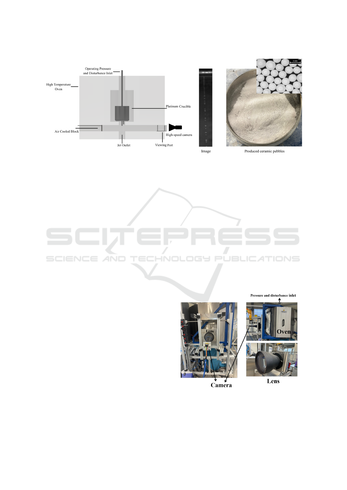
Figure 1: High-temperature KALOS production experimental set-up and the gathered pebbles (Zhang et al., 2024).

The pebbles are then collected at the base of the

tower and transferred to the laboratory for characteri-

zation. An example of the produced pebbles is shown

in Figure 1 on the right.

In addition, Figure 1 also includes an image cap-

tured by the high-speed camera in the middle, demon-

strating the camera system’s ability to clearly capture

the droplets, which is crucial for the measurement

system. The gathered pebbles after cooling (i.e., the

solidiﬁed droplets) are then analyzed in terms of their

sizes and size distributions using a particle analyzer

”HAVER CPA 2-1” by Haver & Boecker, Germany.

The analysis allows for a quantitative validation of the

presented high-speed camera based measurement sys-

tem.

3 COMPUTER VISION BASED

MEASUREMENT SYSTEM FOR

MONITORING THE PEBBLES

FABRICATION

As introduced in the previous section, the quality of

the jet break-up based ceramic pebbles fabrication is

indicated by two measures: the size of the generated

droplets and their coefﬁcient of variation (CV) val-

ues. To ensure the production quality, a measure-

ment system to evaluate the droplet formation in real-

time, focusing on these two measures, has been de-

veloped. The measurement system includes hardware

setup and image processing approaches that are fea-

tured in the following.

3.1 High-Speed Camera System

The major component of the measurement hardware

is a high-speed camera (Optronis CP70-1-M-1000),

which is able to achieve a frame rate of approximately

1000 frames per second (fps) at a maximum resolu-

tion of 1280×1024 pixels. By selecting a region of in-

terest and excluding unnecessary image areas, the im-

age size can be reduced, signiﬁcantly increasing the

maximum possible frame rate. The camera and the

applied telecentric lens are mounted on the side of the

high temperature test facility and monitor the droplet

formation via a port of special glasses combination,

as schematically illustrated in Figure 2. The camera

is arranged in the upper part of the furnace so that it

can observe the droplet formation directly at the cru-

cible nozzle.

Figure 2: High temperature test facility and the applied

high-speed camera system.

A cooled plate is mounted behind the jet to sim-

A Novel Automatic Monitoring and Control System For Induced Jet Breakup Fabrication of Ceramic Pebbles

plify identiﬁcation of the jet and droplets, as it can

provide sufﬁcient light contrast. For the KALOS

process, the optical sensor’s active area measures

8.448 mm × 6.758 mm, with a pixel size of 6.6 µm ×

6.6 µm. Calibration indicates that one pixel in image

coordinates corresponds to an actual size of approxi-

mately 71.94 µm × 71.94 µm. The high-speed camera

allows for an exposure time as short as 2 µs, enabling

clear recording of rapid jet break-up processes and re-

ducing motion blur. To balance for illuminating the

produced droplets while maintaining their spherical

shape, the exposure time was set to 160 µs. The uti-

lized telecentric lens is a specialized optical compo-

nent designed to maintain a consistent magniﬁcation

across varying object distances. Due to its low aber-

ration and stable magniﬁcation properties, it is par-

ticularly well-suited for applications requiring high-

precision dimensional measurements, such as moni-

toring micron-sized droplets. Detailed technical pa-

rameters of the camera and lens are provided in Table

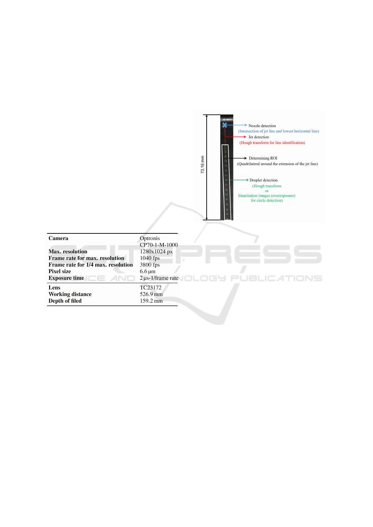
Table 1: Technical details of the high-speed camera and

lens.

For the measurement, the camera system captures

the scene in the form of an image sequence with tem-

porally continuous images. The measurement system

analyses the image sequence to compensate the ran-

dom ﬂuctuation of individual image. The analysing

of one image sequence corresponds to a measuring

cycle.

3.2 Image Processing

After capturing the image sequences, each individual

image of a sequence is processed with image process-

ing approaches to compute the production quality pa-

rameters. The presented measurement system mainly

includes the determining of the nozzle position, the

detection of the jet, and the identiﬁcation of generated

droplets, as schematically depicted in Figure 3. Under

the consideration that the nozzle position is basically

unchanged, the nozzle detection is performed only

once for one image sequence to enhance the compu-

tation efﬁciency. Meanwhile, the detection of the jet

and droplets occurs in all images within the sequence

to ensure an accurate measurement of the production

parameters.

Figure 3: Image processing tasks of the high-speed camera

based measurement system.

Obviously, the most crucial task of this measure-

ment system is to detect the size, amount and position

of the droplets. To accurately localize the droplets and

minimize background noise, the nozzle and jet are de-

tected at ﬁrst, which helps to constrain the region of

interest (ROI) for droplet detection. Only droplets

near the jet extension are identiﬁed, reducing non-

droplet detections from the background and speeding

up the processing to ensure real-time detection. In our

study, the jet is treated as a line with an angle of up to

±10

◦

from the vertical direction. Around the jet line,

ROI is deﬁned as a quadrilateral, whose top and bot-

tom sides are horizontal, while the left and right sides

are parallel to the jet line. The top line of the ROI is at

the end of the jet detection, while the bottom line cor-

responds to the end of the entire image. The left and

right sides are staggered by a certain pixel distance

to the detected jet on the left and right, as presented

in Figure 3. The jet line is detected using the Hough

transform (Hart, 2009). Principally, the nozzle’s lo-

cation is considered the starting point of the jet. For

accuracy, the nozzle is identiﬁed as the intersection

of the jet line with the lowest horizontal line that is

also identiﬁed by the Hough transform. Afterward,

the ROI can be determined and the droplets inside the

ROI are detected by various methods in accordance

with the experient conditions.

Within the detected ROI, the droplets can be iden-

tiﬁed with the help of a Hough transformation or im-

ICINCO 2025 - 22nd International Conference on Informatics in Control, Automation and Robotics

age binarization. The Hough transform is a feature

extraction technique that identiﬁes objects through

a voting process taking place in a parameter space

(Hart, 2009). Initially designed for detecting line seg-

ments in images, the Hough transform is well-suited

for jet detection. Over time, the classical Hough trans-

form has been extended to recognize various shapes,

such as circles (Ballard, 1981). For the introduced

measurement, two form detection methods are inte-

grated: the Hough transform and image binarization.

In the context of droplet detection, the Hough trans-

form demonstrates superior performance in terms of

robustness and accuracy due to its relative insensi-

tivity to individual pixel grey values. Nevertheless,

the precision of localizing detected shapes using the

Hough transform is highly dependent on the regular-

ity of these shapes. When shapes deform for reasons

such as exposure time, the Hough transform’s local-

ization can become biased, signiﬁcantly affecting the

determination of the CV value. To address this is-

sue, the measurement system also contains an alter-

native function for detecting droplets based on binary

images in special cases. For droplet detection using

binary images, each image of a sequence is binarized

by the Otsu threshold selection method, which per-

forms automatic image thresholding based on the grey

value distribution of the image (Otsu, 1979). Subse-

quently, the circle forms are identiﬁed according to

the connectivity of the foreground after binarization

(Haralick and Shapiro, 1992). As mentioned, the bi-

narization detection approach is designed to make up

for the deﬁciency of the Hough transform in deal-

ing with irregular shapes as a consequence of over-

exposure. Therefore, the choice of detection method

in practical application (KALOS process) depends on

the exposure time. The system switches to this alter-

native method when the required exposure time ex-

ceeds 500 µs.

For the measurement system, the droplet diame-

ter can be directly introduced by the circle detection

approaches, while the CV value needs computing fol-

lowing in line with the deﬁnition of equation 1. The

standard deviation of the droplet spacing (σ(s)) is de-

noted as:

σ(s) =

N − 1

∑

i=1

− µ(s))

, (2)

and the average spacing µ(s) is computed as:

µ(s) =

∑

i=1

(3)

Before computing the CV value, the detected droplets

are rearranged from top to bottom according to their

positions, then the distance between neighbouring

droplets are calculated and noted as s

. Hereby, i rep-

resents the ith droplet spacing of the N spacing for

N + 1 droplet detections. To compensate for the ﬂuc-

tuations of the results based on individual images, the

measurement system outputs the average CV value of

an image sequence with M images as:

σ =

∑

j=1

σ( j)

. (4)

4 AUTOMATIC CONTROL

SYSTEM

As introduced in the previous sections, the CV value

indicates the regularity of the molten jet break-up and

is thus the most crucial parameter in ceramic pebble

production. The present control system applies the

CV value as the control foundation. Albeit theoret-

ically, frequencies within a certain range should en-

hance the jet break-up regularity (thereby lowering

the CV value), empirical studies have demonstrated

that the CV value’s response to driving frequency can

be irregular (Leys et al., 2019). Even within the effec-

tive frequency range, instances indicate that the CV

value abruptly increases at several frequencies. It is

hypothesized that these frequencies correspond to res-

onances within the system, which subsequently cause

a more irregular jet break-up. To ensure the regularity

of the droplets generation and the quality of the peb-

bles fabrication, a real-time control system for adjust-

ing the driving frequency is necessary. Once the CV

value surpasses a predetermined threshold, the control

system is able to adapt the frequency to facilitate the

stability of the droplet generation. With the integra-

tion of the control system, the ceramic pebbles fabri-

cation can be automatically monitored and controlled

in real-time. The complete schematic representation

of this process is shown in Figure 4.

As illustrated in Figure 4, the measured CV value

is transferred from the measurement system to the

control system, which then regulates the driving fre-

quency. Afterward, the to be adjusted frequency value

is passed to LabVIEW, which can implement the ad-

justment of the process parameter according to the

control system. In addition, LabVIEW also displays

the process parameter and the measurement results in

real time. Therefore, LabVIEW is interpreted as a

visualization and operating system for the entire pro-

duction. The measurement system, the control sys-

tem, and the operating system work together to real-

ize the closed-loop monitoring and control of the en-

tire production process. This section concentrates on

A Novel Automatic Monitoring and Control System For Induced Jet Breakup Fabrication of Ceramic Pebbles

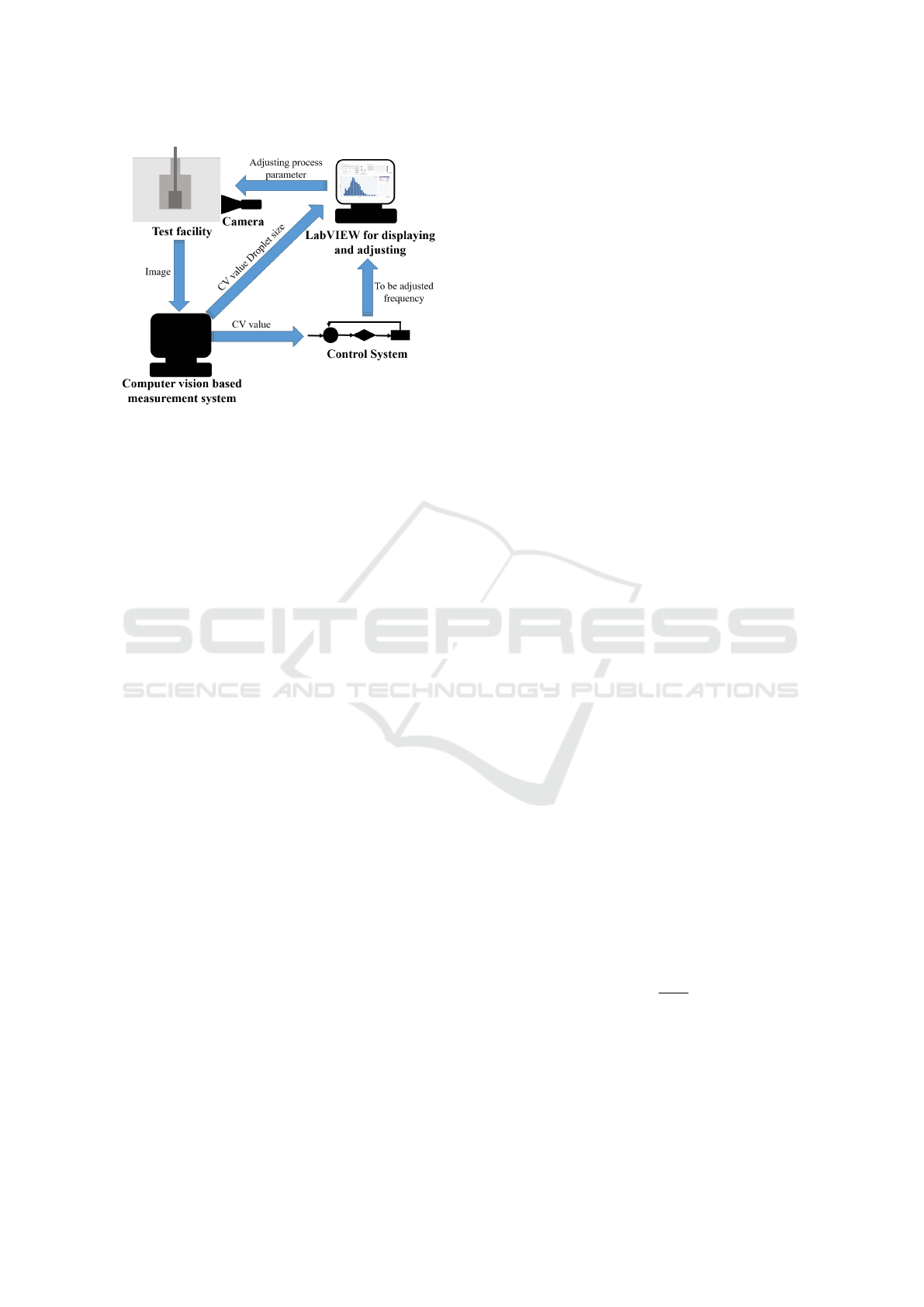
Figure 4: Schematic of the introduced measurement sys-

tems and control systems for monitoring and controlling the

KALOS process.

the control system.

Figure 5 provides an overview of the control logic.

A small value of CV indicates a sufﬁcient quality of

the droplet generation. When the measured CV value

exceeds a predeﬁned threshold, the current driving

frequency requires adjustment. In line with the the-

ory, the optimal frequency for a speciﬁc production

should not vary signiﬁcantly from the principal opti-

mum. Typically, each process setup has several ﬁxed

optimal driving frequencies, and adjustments are usu-

ally minor. Thus, a range of variation is deﬁned in the

control system as well. If the frequency adjustments

fail to reduce the CV value to the desired threshold

within acceptable limits, the system will alert the op-

erator to inspect the nozzle for potential issues. Un-

der these circumstances, the problem is most likely

caused by the nozzle (for instance, the nozzle being

affected by the melt), not the driving frequency of the

process.

Initially, the system selects an initial frequency

determined by theory and empirical observation. In

the KALOS process this initial frequency is set as

1000 Hz. The measuring system measures then the

corresponding CV value at 1000Hz. Thereafter, the

system chooses a frequency between 750 and 1000 Hz

and measures the corresponding CV value. Subse-

quently, a frequency between 1000 Hz and 1250 Hz

is chosen and the corresponding CV value is mea-

sured. Based on these three known frequencies and

corresponding measured CV values, a quadratic poly-

nomial is ﬁtted to more accurately determine the opti-

mal frequency value. The minimum point of the com-

puted quadratic polynomial (i.e., the smallest approx-

imated CV value) is calculated and its corresponding

frequency is utilized as a new driving frequency. After

measuring the CV value for this frequency, the poly-

nomial ﬁt is repeated based on four points and the

driving frequency is again adapted to the frequency of

the new minimal CV value. This iterative procedure

stops when the frequency change signiﬁcantly slows

down, because under this condition, adding more CV

values at additonal frequencies to the polynomial ﬁt-

ting provides only a slight beneﬁt. The system then

switches to a more sophisticated algorithm to ﬁnd the

optimum. With the help of polynomial ﬁtting, the

control system can limit the regulation range within a

certain area, which beneﬁts the regulation efﬁciency

and reduces the control time. The system regards

the minimizer of the quadratic polynomial as the ini-

tial value to determine the ﬁnal optimal frequency by

applying the global optimum ﬁnding solution. The

applied global search algorithm is the simulated an-

nealing (van Laarhoven and Aarts, 1987). Compared

to other global optimum searching methods, such as

the Burg Algorithm (Orfanidis, 1985) and the Parti-

cle Swarm Optimization (Pedersen, 2010), the sim-

ulated annealing algorithm shows its merits in the

global search capability, the high adaptability, and its

simple implementation. The Burg Algorithm is pri-

marily used for spectral estimation and signal pro-

cessing, which is suitable for handling time series

data and not appropriate for combinatorial optimiza-

tion problems (Vos, 2013).The Particle Swarm Opti-

mization optimizes problems by simulating group be-

havior, which is adequate for continuous optimization

problems (Bonyadi and Michalewicz, 2017). Since

PSO shows accurate performance in searching large

spaces, it can get trapped in local optima.

The technique of simulated annealing is based on

the parallelism between the problem of ﬁnding the

minimum of a function and the phenomenon of an-

nealing in statistical mechanics (Banchs, 1997). Af-

ter measuring the CV value corresponding to the ini-

tial frequency, which is determined by the polynomial

ﬁtting, the simulated annealing then randomly gener-

ates a new solution in the neighborhood of the current

solution. Subsequently, the CV value of the new so-

lution is compared with the last CV value. If the new

CV value is smaller than the previous one, the new

frequency is accepted. Otherwise, a probability deter-

mined by the Metropolis criterion (Metropolis et al.,

1953) is computed, as:

P = exp



−

∆CV



, (5)

where ∆CV is denoted as the CV value difference and

f is the utilized frequency. The new solution with

a higher CV value is accepted with this probability.

Afterward, the driving frequency is adjusted again by

a step of

new

= α · f . (6)

ICINCO 2025 - 22nd International Conference on Informatics in Control, Automation and Robotics

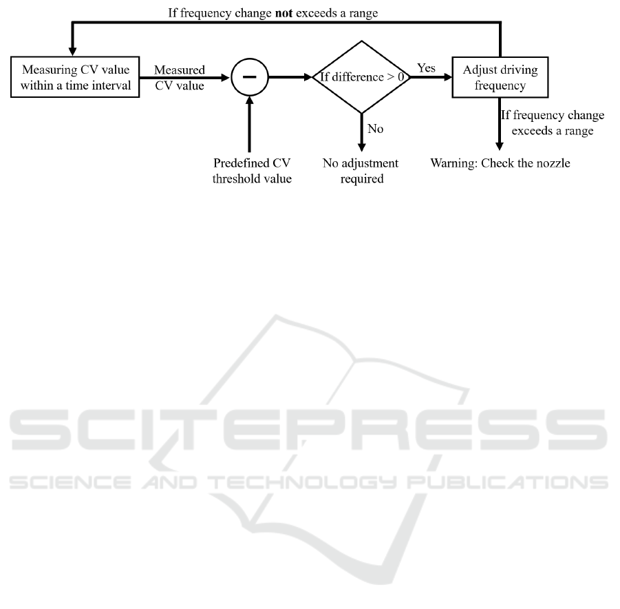
Figure 5: Schematic of the control logic.

For the present control system, α is deﬁned as a ran-

dom value from a normal distribution with the av-

erage value of 0 and a standard deviation of 0.01.

The iteration stops when the frequency reaches a cer-

tain threshold or the maximum number of iterations

is reached. The control system then ouputs the fre-

quency with the lowest found CV value. By imple-

menting these steps, the simulated annealing (SA) al-

gorithm can effectively escape local optima (Dela-

haye et al., 2018). Nevertheless, for a real-time con-

trol system, where an optimum is desired in a pos-

sible short time, the SA algorithm alone without re-

stricting the search area in advance is inappropriate,

since it requires costly computational time to ensure

its functionality. Thus, we combine a polynomial ﬁt-

ting together with SA algorithm to realize a sufﬁcient

accuracy in an acceptable time.

If the control system is not activated to function at

the very beginning, but is triggered by a CV value ex-

ceeding the threshold during production, the polyno-

mial ﬁtting is initialized to the current frequency, fol-

lowed by a new frequency randomized within 250 Hz

to the left and right of it.

In addition, in order to ensure that the KALOS

process has sufﬁcient response time to frequency

changes, the measurement system usually captures

several image sequences before conducting the mea-

surement, which is controlled by the measurement

signal.

5 RESULTS AND DISCUSSION

The image processing techniques and control system

are outlined in the previous sections. This section

presents and discusses the results of these methods.

For the computer vision based measurement system,

the two crucial parameters, i.e., the CV values and the

molten ceramic droplets’ diameters, are computed.

For the purpose of validating the performance of the

high-speed camera based measurement system, the

gathered pebbles after cooling are analyzed in terms

of their diameters, which can be compared with the

measurement outputs to evaluate the accuracy of the

system. For the control system, the control process

and the intermediate frequencies are visualized to fol-

low the frequency adjustments.

5.1 Computer Vision Based

Measurement System

At ﬁrst, droplets are generated by applying driving

frequencies ranging from 0 to 5000 Hz to provide an

overview of the frequency’s effects. According to ex-

tensive experimental data and theoretical foundations,

frequencies above 3000 Hz barely affect the jet break-

up. Thus, frequency ramps from 0 to 5000 Hz were

used to study the frequency effects, ensuring the en-

tire range of inﬂuence was covered. Figure 6 displays

images of the jet break-up captured by the high-speed

camera at a frame rate of 500 fps over three minutes.

With a gradually increasing driving frequency, the

average diameter increases and then decreases. The

change in the CV value is not easily discernible from

the ﬁgure. The smallest CV value is observed at a

driving frequency of around 1000 Hz. To achieve a

more visible observation of the impact of the driv-

ing frequency on the CV value and droplet diame-

ter, the results of the image processing are presented

in Figure 7. The horizontal axis represents the driv-

ing frequency, while the vertical axis shows the CV

and diameter, respectively. Each green point corre-

sponds to the CV value or median diameter based on

a single image (frame) generated by the correspond-

ing frequency. For statistical observation, the data

are smoothed by a robust linear regression (Andersen,

2008) over a window of 200 frames that are presented

by the black lines in the ﬁgure.

A Novel Automatic Monitoring and Control System For Induced Jet Breakup Fabrication of Ceramic Pebbles

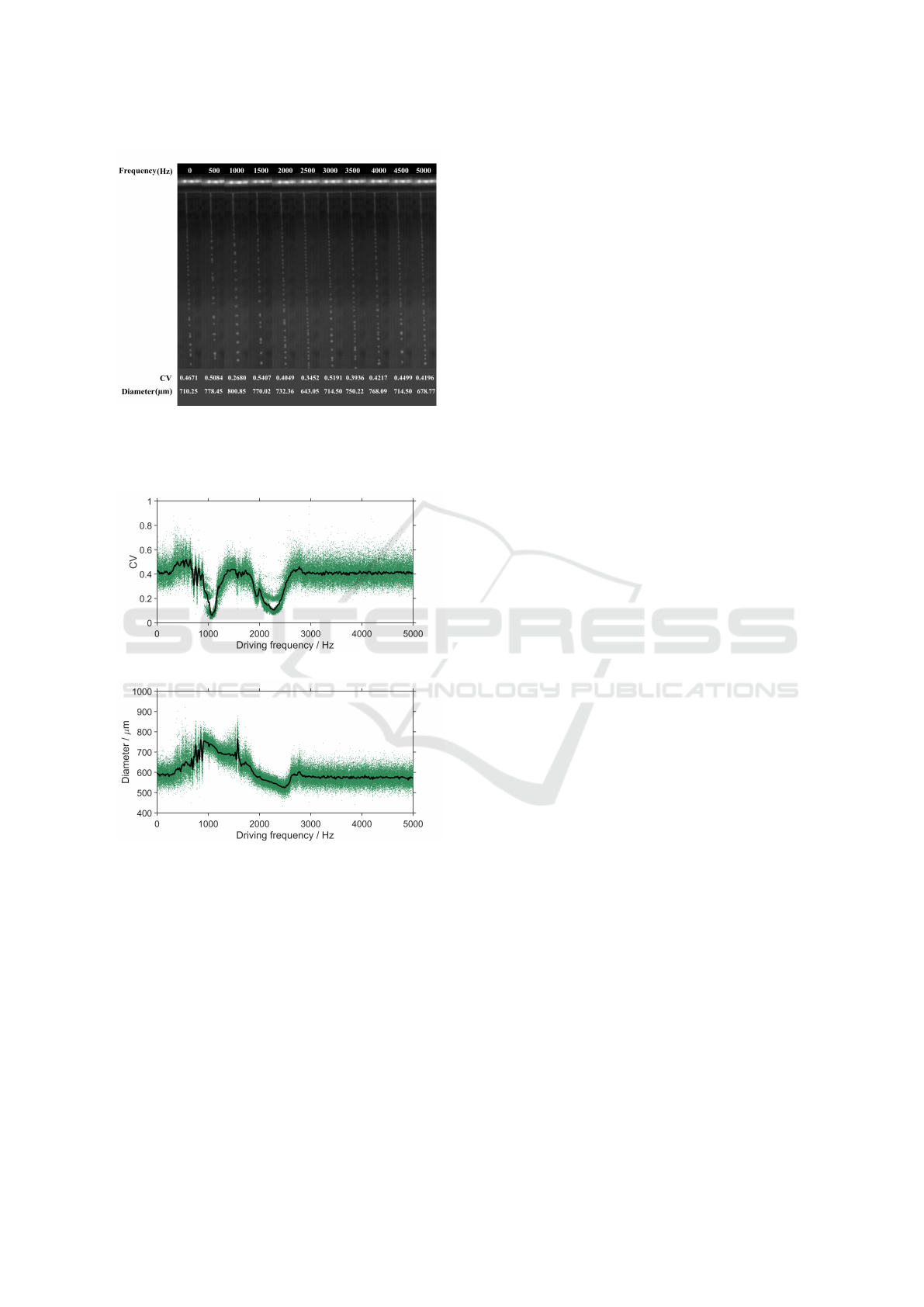
Figure 6: Effect of the driving frequency on the appearance

the molten ceramic jet break-up. The corresponding CV

values and droplet diameters (in µm), calculated by the im-

age processing algorithms, are shown at the bottom.

(a)

(b)

Figure 7: Output of the measurement system. (a) The CV

value and (b) The median diameter of the droplets.

As revealed by Figure 7(a), frequencies between

approximately 800 Hz and 2600 Hz affect the jet

break-up, and in general, two minima exist: one

around 1000 Hz and another at around 2300 Hz. Be-

tween these two minima, internal resonances disturb

the jet break-up, as indicated by the irregular jet

break-up images at 1500 Hz and 2000 Hz in Figure

6. As for the impact of the driving frequency on the

droplet diameter, at a driving frequency of 1000 Hz,

droplets with diameters of approximately 750 µm are

formed, while at 2500 Hz, droplets with diameters of

550 µm are produced. Apparently, the diameter de-

crease linearly from 1000 Hz to 2500 Hz. Again, res-

onances in the system are evident around 1500 Hz,

where there is a greater variation around the smoothed

data value. As proved by Figure 7, the optimum of

the CV value occurs at a driving frequency of approx-

imately 1000 Hz, which is also the initial value of the

control system. Thereafter, we also conducted experi-

ments to investigate the droplet generation at the driv-

ing frequency of 1000 Hz with respect to the droplet

diameter.

The measured droplet diameters and the analyzed

pebble diameters are presented in Figure 8. In Fig-

ure 8 (a), the high-speed camera based measured di-

ameters are depicted in a green histogram in inter-

vals of 5 µm with an approximated normal probabil-

ity density distribution. The black dashed line stands

for the diameter with the highest probability density,

while the orange dashed line represents the average

diameter of the best ﬁtting normal distribution. As

shown in the ﬁgure, the diameter with the highest

probability occurs in the interval 760 µm to 765 µm,

and the average value of the ﬁtted normal distribu-

tion is 732.05 µm. The vast majority of the produced

droplets are between 500 and 1000 µm in diameter.

To validate the adequacy and accuracy of the pro-

posed measurement system, solidiﬁed pebbles after

cooling are collected and physically analyzed by a

particle analyzer for determining their sizes and dis-

tribution, as shown in Figure 8 (b). In the ﬁgure, the

histogram with larger intervals depicts the distribution

of pebble diameters, and the red line marks the cu-

mulative distribution of the pebble diameter. Accord-

ing to the analysis the pebble diameters are primarily

focused between 600 µm and 800 µm, and the most

probable diameter around 750 µm, matching the mea-

sured size of the generated droplets shown in Figure 8

(a). Taking the solidiﬁcation effects and the physical

deformation of the droplets during falling into consid-

eration, which can result in slightly altering of the size

between the droplets and the solid pebbles, the peb-

ble size distribution results and the image processing

of the jet break-up are in strong agreement, thereby

validating the measurement system’s accuracy.

5.2 Control System

In order to present the regulation process of the con-

trol system more clearly, we select an experiment for

validation and show its CV value / frequency curve in

Figure 9. In the experiment, the driving frequency

varies from 0 to 5000 Hz, and the images are cap-

tured with a framerate of 500 fps. Similar to Figure

7 (a), green points represent the CV values for sin-

ICINCO 2025 - 22nd International Conference on Informatics in Control, Automation and Robotics

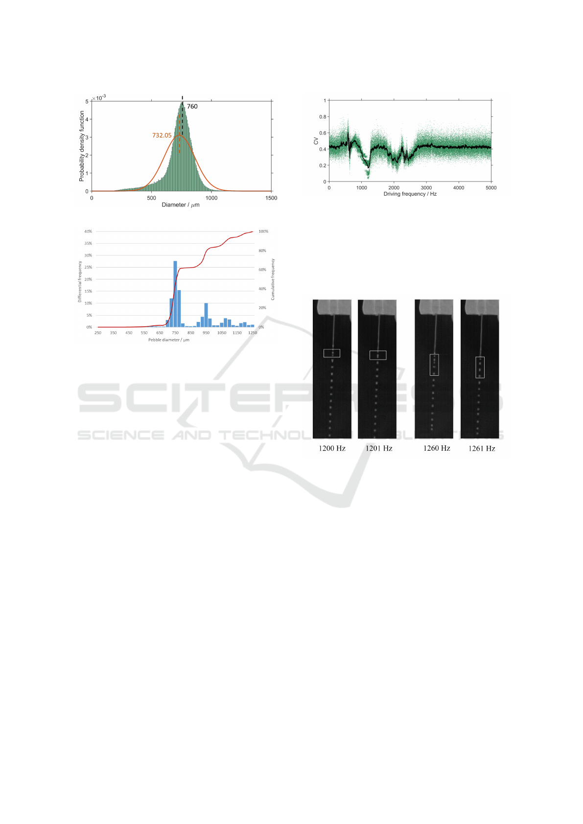
(a)

(b)

Figure 8: Diameter of droplets and gathered pebbles at the

driving frequency of 1000 Hz. (a) Measured droplet diame-

ters and its distribution. (b) Measured diameter distribution

of the pebbles provided by particle analyzer HAVER CPA

2-1.

gle frames generated by the corresponding frequency,

while the black line illustrates the smoothed version

over a window of 200 frames. Obviously, compared

to the experiment displayed in ﬁgure 7, this experi-

ment is more difﬁcult to modulate since its CV distri-

bution is more diffuse with a signiﬁcant ﬂuctuation.

Moreover, the CV of this experiment ﬂuctuates dras-

tically at the two local minimum points, i.e., around

1000 Hz and 2000 Hz. Especially around 1000 Hz,

the local CV distribution seems disconnected due to

the local large variation of CV values, which is pri-

marily caused by suspected internal resonances that

lead to irregular jet break-up. In order to explain the

situation more visually, two sets of images taken at

adjacent frequencies are shown in Figure 10.

Figure 10 shows four images taken at different fre-

quencies. Apparently, the difference occurs when the

droplets are ﬁrst generated. For example, at 1200 Hz,

the droplets in the white box are detected as two,

whereas at 1201 Hz, in essentially the same image po-

sition, the two droplets converge into one large one.

A more pronounced difference can be observed at

1260 Hz and 1261 Hz, where the droplet generation is

unstable due to the irregularity of jet break-up, which

affects the CV value. This phenomenon highlights the

Figure 9: Plot of CV value versus driving frequency for one

experiment. Frequency ramp from 0-5000 Hz

need for a control system to manage unknown system

responses. In addition, with the help of the waiting

time in the control system for waiting the response,

some random irregularity can be attenuated to some

extent.

Figure 10: Captured images of adjacent frequencies.

As described in Section 4, we select at ﬁrst three

data points around 1000 Hz and approximate a poly-

nomial approach to these points. Afterward, the input

data are updated using the local minimum of each ﬁt-

ted polynomial. The process is detailed in Figure 11.

As presented by the ﬁgure, the polynomial ﬁtting is

repeated ﬁve times and stops when the curves only

barely vary. The local minimum of the last curve is

considered as the inital point for the following global

optimization algorithm.

Using the polynomial ﬁtting output as an initial

point, the control system performs the simulated an-

nealing algorithm to ﬁnalize the optimal frequency.

The temporal results of the algorithm during the reg-

ulation are shown in Figure 12 and the corresponding

detailed values for each adjustment are listed in the

Table 2. The control system ﬁrst adjusts the frequency

around the initial value (1114 Hz) and then measures

the CV value. Subsequently, according to the algo-

rithm, all frequencies resulting in smaller CV values

A Novel Automatic Monitoring and Control System For Induced Jet Breakup Fabrication of Ceramic Pebbles

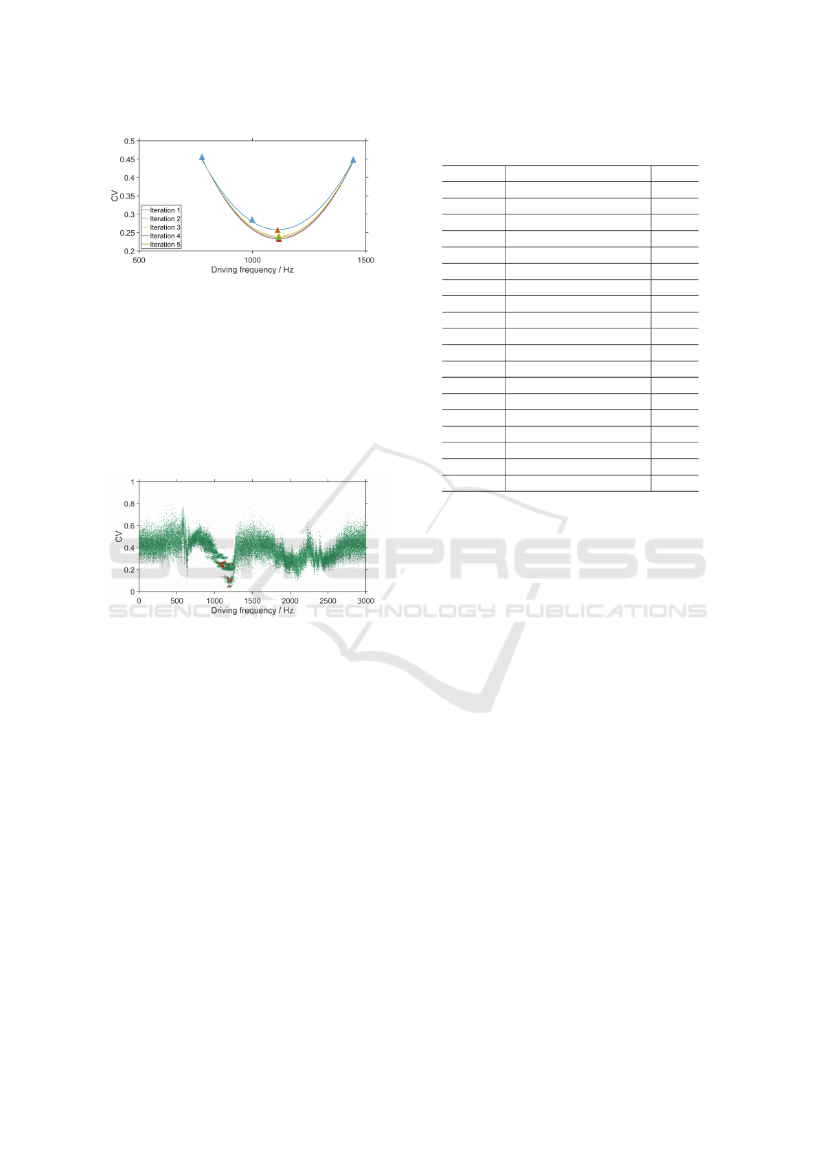
Figure 11: Process of polynomial ﬁtting. Different curves

represent different iterations. The triangles in the image are

the data points for each ﬁtting, whose colors also identify

the number of iteration.

are updated as the new input. Frequencies leading

to larger CV values are only accepted with a certain

probability to ensure that the local optimum solution

is skipped. It should be noted that in Table 2 only the

steps that are updated by new frequencies are listed.

In several steps, the frequencies are not updated be-

cause of increasing CV values.

Figure 12: Temporal results of the control output by the

simulated annealing algorithm. Green points denote mea-

surement points and red asterisks indicate the data points

that are scanned by regulation.

At ﬁrst, the control system adjusts the frequency

at around 1110 Hz, however, the CV value does not

decrease signiﬁcantly. Therefore, the system reduces

the frequency to around 1000 Hz. Although the CV

value ﬂuctuates, none of them reached the system’s

threshold, 0.2. Subsequently, the system continues to

move the frequency range to around 1200 Hz, where

the system detects a very low CV value (already ap-

proaching the optimal solution). Thereafter, the sys-

tem still tries to vary the driving frequency, but none

of the resulting CV values reach below this CV value.

Additionally, the system starts to converge, i.e., the

difference between the measured CV value and the

detected minimum value becomes smaller, and then

the iteration stops.

Despite the fact that the local minimum has been

roughly determined previously by polynomial ﬁtting,

the whole control process lasts for several dozen it-

erations, and since each iteration also requires a cor-

Table 2: Driving frequency and CV value of each control

step.

Iteration Driving frequency (Hz) CV

1 1114 0.238

2 1109 0.227

3 1072 0.253

4 1188 0.115

5 1184 0.253

6 1089 0.263

7 1095 0.232

8 1040 0.263

9 1076 0.249

10 1117 0.265

11 1139 0.274

12 1168 0.218

13 1212 0.100

14 1218 0.111

15 1240 0.245

16 1174 0.041

17 1171 0.130

18 1179 0.092

19 1190 0.052

responding waiting time, the overall duration is the

product of the waiting time and the number of itera-

tions. The processing time of each image sequence

is about 2 to 3 s, thus, the process lasts about 3 min,

which is acceptable in the KALOS process. Obvi-

ously, without polynomial ﬁtting, the whole regula-

tion will take much longer, signiﬁcantly affecting the

production.

6 CONCLUSIONS

The paper presents a novel high-speed camera based

measurement and control system that aims to analyze

and control the production of lithium pebbles for fu-

sion reactors automatically. The system, which in-

corporates image processing techniques, allows for

real-time monitoring of the droplet generation process

and measuring the droplet diameters and the normal-

ized standard deviation of droplet spacing (CV). The

CV value is considered as the most crucial parame-

ter to indicate the fabrication performance, since it

directly indicates the regularity of the jet break-up.

Moreover, the CV value also guides the adjustment

of the driving frequency of the control system. Ac-

cording to the molten jet break-up theory discussed in

the second section, a low CV value indicates a regular

and stable jet break-up, which is desirable for produc-

tion. Owing to the introduced measurement system,

the study enables the investigation into the inﬂuence

ICINCO 2025 - 22nd International Conference on Informatics in Control, Automation and Robotics

of the driving frequency on the CV value and droplet

diameter. The experiments are conducted with both

varying driving frequency, which provides a broad

overview of ceramic droplet production, and a certain

frequency. As revealed by the results, the driving fre-

quency signiﬁcantly affects production performance

within a certain range, with the optimal frequency for

the utilized nozzle being around 1000 Hz. The exper-

iment under 1000 Hz driving frequency is further ex-

amined in detail, and the solid ceramic pebbles under

this condition are collected and analyzed by a parti-

cle analyzer. By comparing the measured droplet di-

ameters with the analyzed pebble diameters, the accu-

racy and reliability of the computer vision based mea-

surement system has been proved. Given that gener-

ation frequency is a critical parameter for controlling

droplet production, the measurement system proves

essential for selecting the initial frequency and mak-

ing further adjustments. If the CV value exceeds a

certain value, the driving frequency needs adjustment

implemented by the control system to maintain an op-

timal CV value. For the adjustment, the control sys-

tem performs a polynomial ﬁtting at ﬁrst to roughly

deﬁne an initial minimum, which is regarded as input

to the subsequent global optimization algorithm. The

utilized algorithm is the simulated annealing, which

is widely applied to search global optimum. Accord-

ing to the performance of the algorithm on the exper-

iment, the control system is able to realize real-time

control of the system.

Our experiments with the described settings

demonstrate the effectiveness of the proposed auto-

matic system in monitoring and controlling ceramic

pebble production. Future research will focus on eval-

uating the system’s robustness under different condi-

tions. Additionally, we plan to enhance the image

processing techniques to analyze the generation and

motion velocity of the produced droplets. By ex-

amining the generation speed, we can calculate the

quantity of droplets, which will help estimate the ef-

ﬁciency of raw material usage.

ACKNOWLEDGEMENTS

This work has been carried out within the framework

of the EUROfusion Consortium, funded by the Eu-

ropean Union via the Euratom Research and Training

Programme (Grant Agreement No 101052200 — EU-

ROfusion).

REFERENCES

Andersen, R. (2008). Modern methods for robust regres-

sion. Sage University Paper Series on Quantitative

Applications in the Social Sciences, pages 1654–1662.

Ballard, D. (1981). Generalizing the hough transform to de-

tect arbitrary shapes. Pattern Recognition, 13(2):111–

122.

Banchs, R. E. (1997). Simulated annealing. Technical re-

port, The University of Texas at Austin.

Bonyadi, M. R. and Michalewicz, Z. (2017). Particle

swarm optimization for single objective continuous

space problems: A review. Evolutionary Computa-

tion, 25(1):1–54.

Cai, J., Xu, G., Lu, H., Xu, C., Hu, Y., Cai, C., and

Suo, J. (2022). Preparation of tritium breeding li2tio3

ceramic pebbles via newly developed piezoelectric

micro-droplet jetting. Journal of the American Ce-

ramic Society, 105.

Delahaye, D., Chaimatanan, S., and Mongeau, M. (2018).

Simulated annealing: From basics to applications.

pages 1–35.

Haralick, R. M. and Shapiro, L. G. (1992). Computer

and Robot Vision, Volume I, pages 28–48. Addison-

Wesley.

Hart, P. E. (2009). How the hough transform was in-

vented [dsp history]. IEEE Signal Processing Mag-

azine, 26(6):18–22.

Hern

andez, F. A., Arbeiter, F., Boccaccini, L. V., Bubelis,

E., Chakin, V. P., Cristescu, I., Ghidersa, B. E.,

Gonz

alez, M., Hering, W., Hern

andez, T., Jin, X. Z.,

Kamlah, M., Kiss, B., Knitter, R., Kolb, M. H. H.,

Kurinskiy, P., Leys, O., Maione, I. A., Moscardini, M.,

adasi, G., Neuberger, H., Pereslavtsev, P., Pupeschi,

S., Rolli, R., Ruck, S., Spagnuolo, G. A., Vladimirov,

P. V., Zeile, C., and Zhou, G. (2018). Overview of the

hcpb research activities in eurofusion. IEEE Transac-

tions on Plasma Science, 46(6):2247–2261.

Heuser, J., Kolb, M., Bergfeldt, T., and Knitter, R. (2018).

Long-term thermal stability of two-phased lithium or-

thosilicate/metatitanate ceramics. Journal of Nuclear

Materials, 507:396–402.

Knitter, R., Alm, B., and Roth, G. (2007). Crystallisa-

tion and microstructure of lithium orthosilicate peb-

bles. Journal of Nuclear Materials, 367-370:1387–

1392. Proceedings of the Twelfth International Con-

ference on Fusion Reactor Materials (ICFRM-12).

Knitter, R., Chaudhuri, P., Feng, Y., Hoshino, T., and Yu, I.-

K. (2013). Recent developments of solid breeder fab-

rication. Journal of Nuclear Materials, 442(1, Supple-

ment 1):S420–S424. 15th International Conference on

Fusion Reactor Materials.

Leys, O., Bergfeldt, T., Kolb, M. H., Knitter, R., and

Goraieb, A. A. (2016). The reprocessing of ad-

vanced mixed lithium orthosilicate/metatitanate tri-

tium breeder pebbles. Fusion Engineering and De-

sign, 107:70–74.

Leys, O., Leys, J. M., and Knitter, R. (2021). Current status

and future perspectives of eu ceramic breeder develop-

ment. Fusion Engineering and Design, 164:112171.

A Novel Automatic Monitoring and Control System For Induced Jet Breakup Fabrication of Ceramic Pebbles

Leys, O., Waibel, P., Matthes, J., and Knitter, R. (2019).

Ceramic pebble production from the break-up of a

molten laminar jet. In Proc of ILASS Europe 2019:

29th Conference on Liquid Atomization and Spray

Systems.

Metropolis, N., Rosenbluth, A. W., Rosenbluth, M. N.,

Teller, A. H., and Teller, E. (1953). Equation of state

calculations by fast computing machines. The Journal

of Chemical Physics, 21(6):1087–1092.

Orfanidis, S. J. (1985). Optimum signal processing : an

introduction. Macmillan, New York.

Otsu, N. (1979). A threshold selection method from gray-

level histograms. IEEE Transactions on Systems,

Man, and Cybernetics, 9(1):62–66.

Park, Y.-H., Cho, S., and Ahn, M.-Y. (2014). Fabrication

of li2tio3 pebbles using pva–boric acid reaction for

solid breeding materials. Journal of Nuclear Mate-

rials, 455(1):106–110. Proceedings of the 16th In-

ternational Conference on Fusion Reactor Materials

(ICFRM-16).

Pedersen, M. E. H. (2010). Good parameters for particle

swarm optimization.

van Laarhoven, P. J. M. and Aarts, E. H. L. (1987). Sim-

ulated annealing : theory and applications. Kluwer

Academic Publishers.

Vos, K. (2013). A fast implementation of burg’s method.

pages 2–4.

Zhang, M., Leys, O., Vogelbacher, M., Knitter, R., and

Matthes, J. (2024). A high-speed camera-based mea-

surement system for monitoring and controlling the

induced jet break-up fabrication of advanced ceramic

breeder pebbles. The International Journal of Ad-

vanced Manufacturing Technology.

ICINCO 2025 - 22nd International Conference on Informatics in Control, Automation and Robotics