Enhancing Pharmaceutical Batch Processes Monitoring with Predictive

LSTM-Based Framework

Daniele Antonucci

1,2

, Davide Bonanni

, Domenico Palumberi

, Luca Consolini

and Gianluigi

Ferrari

Department of Information Engineering and Architecture, University of Parma, Via delle Scienze 181/a, Italy

Department of Electrical and Information Engineering , Politecnico of Bari, Via Re David 200, 70125 Bari, Italy

GlaxoSmithKline s.p.a., Strada Provinciale Asolana, 90, San Polo Torrile, Parma, Italy

Department of Information Engineering and Architecture, Universit

a di Parma, Via delle Scienze 181/a, Parma, Italy

Keywords:

Anomaly Detection, Predictive Maintenance, Machine Learning, Artiﬁcial Intelligence, AutoEncoder,

Time-Series Forecasting, Hyperparameter Optimization, Fault Detection.

Abstract:

Monitoring industrial processes and understanding deviations is critical in ensuring product quality, process

efﬁciency, and early detection of anomalies. Traditional methods for dimensionality reduction and anomaly

detection, such as Principal Component Analysis (PCA) or Partial Least Squares (PLS), often struggle to

capture the complex and dynamic nature of batch data. In this study, we propose a novel approach that

combines an AutoEncoder (AE), based on Long Short-Term Memory (LSTM) layers, with a rolling threshold

for anomaly evaluation. Unlike conventional threshold methods that rely on global statistical parameters, the

applied threshold leverages rolling median and rolling Median Absolute Deviation (MAD) to adaptively detect

deviations, making it more resilient to outliers and distribution shifts. The LSTM-AE demonstrates superior

performance in anomaly detection with respect to PCA and more recent model approaches, speciﬁcally for

the reference dataset, obtained from a GlaxoSmithKline (GSK) production plant. Additionally, an LSTM

regression model is employed to forecast future data points, which are then fed into the LSTM-AE to enable

a predictive approach. This framework leverages the temporal dependencies captured by LSTM layers and

reconstruction efﬁciency of the AE, facilitating a predictive anomaly detection in real-world applications.

1 INTRODUCTION

An anomaly is an unexpected deviation from nor-

mal system behavior, representing data points or

events that stray from the operational baseline. These

anomalies can indicate critical issues—such as faults,

errors, or fraudulent activities—that may lead to de-

graded performance, failures, safety risks, or ﬁnancial

losses. Pharmaceutical processes, in particular, are

complex and strictly regulated. Anomalies in these

settings can result from equipment malfunctions, en-

vironmental changes, human errors, or variations in

raw material properties, making swift detection essen-

tial for maintaining process integrity. However, de-

tecting anomalies is particularly challenging in batch

operations, which involve dynamic, stage-speciﬁc be-

haviors and batch-to-batch variability (see (Majozi,

2009)). An anomaly in one stage might be typi-

cal in another, further complicating detection. Addi-

tionally, batch-to-batch variability—driven by factors

like raw material quality, environmental conditions,

or equipment wear—further obscures the identiﬁca-

tion of subtle anomalies (Mockus et al., 2015).

Over the past decade, various data-driven methods

have been employed for anomaly prediction. Tradi-

tional statistical techniques, such as PCA (Greenacre

et al., 2022) and PLS (Pirouz, 2006), have been

widely used, even though their linear nature lim-

its their ability to capture non-linear interactions in

batch data. Extensions like kPCA (Sch

olkopf et al.,

1997) and non-linear PLS have been developed but

often come with high computational costs. Recent

advances in Machine Learning (ML) and Deep Learn-

ing (DL)—particularly AutoEncoders (AEs) and Re-

current Neural Networks (RNNs) (Aghaee et al.,

2024)—have shown promise in capturing both non-

linear patterns and temporal dependencies in dynamic

systems.

Antonucci, D., Bonanni, D., Palumberi, D., Consolini, L. and Ferrari, G.

Enhancing Pharmaceutical Batch Processes Monitoring with Predictive LSTM-Based Framework.

DOI: 10.5220/0013665500003982

Paper published under CC license (CC BY-NC-ND 4.0)

In Proceedings of the 22nd International Conference on Informatics in Control, Automation and Robotics (ICINCO 2025) - Volume 1, pages 15-24

ISBN: 978-989-758-770-2; ISSN: 2184-2809

This paper introduces a robust framework that

combines LSTM and AE methodologies (detailed in

Section 3) for batch process monitoring. It demon-

strates improved performance in managing the com-

plex dynamics of batch process monitoring in com-

parison to traditional approaches (discussed in Sec-

tion 4.1). Furthermore, a customized threshold mech-

anism, based on rolling median and Median Abso-

lute Deviation (MAD) is implemented to enhance

anomaly detection accuracy and reduce false posi-

tives. Notably, the framework also employs an LSTM

regression model to predict future process variables,

which are subsequently fed into the AE to enable pre-

dictive anomaly detection.

Paper Outline

In Section 2, we discuss existing approaches for

anomaly detection in batch processes, including sta-

tistical and ML-based methods, and we outline the

motivation behind our proposed framework. Sec-

tion 3 introduces the architecture, implementation,

and integration of our framework composed by an

LSTM-AE model alongside the LSTM regression

model, designed for both real-time monitoring and

prediction. The training and testing of these models

utilize batch process data sourced from the pharma-

ceutical company GSK (as detailed in Section 3.1).

Section 4 describes the experimental setup, evaluation

metrics, and provides a comparative analysis of our

approach against alternative methods. Finally, Sec-

tion 5 concludes the paper by summarizing key ﬁnd-

ings, discussing their implications, and suggesting fu-

ture research.

2 LITERATURE REVIEW

Despite the inherent non-linearity of industrial pro-

cesses, PCA remains popular for process modeling

due to its simplicity and ease of use (Russell et al.,

2000). An alternative for batch processes, as shown

in (Jeffy et al., 2018), employs a multi-way PCA tech-

nique by aligning and concatenating batches into an

unfolded 2D matrix, suited for following transforma-

tions. The advantages of PCA in industrial applica-

tions include robust irregularity detection even with

sparse data, scalability for process efﬁciency, and ease

of interpretation for real-time monitoring and control.

Transitioning from linear to non-linear methods

introduces challenges in deploying optimized, inter-

pretable models for fault detection in highly non-

linear systems. Non-linear techniques offer enhanced

modeling capabilities but often demand greater com-

putational resources and larger training datasets. For

instance, Kernel PCA (kPCA)—presented in (Choi

et al., 2005)—addresses linear PCA’s limitations by

modeling complex non-linear relationships. How-

ever, kPCA requires signiﬁcant computational re-

sources due to the need to compute and store a kernel

matrix that scales quadratically with the number of

samples, and its high-dimensional feature space can

complicate interpretation.

Building on these non-linear techniques, methods

such as one-class Support Vector Machine (SVM)

(Li et al., 2003) and Support Vector Data Descrip-

tion (SVDD) (Zhao et al., 2013) have been adopted to

enhance anomaly detection. Both these methods use

kernel functions to map data into a high-dimensional

space based solely on fault-free samples, with a key

distinction in the boundary: one-class SVM con-

structs a hyperplane while SVDD deﬁnes a hyper-

sphere. In (Inoue et al., 2017), one-class SVM is

compared with Deep Neural Networks (DNNs) for

detecting anomalies in the context of a water treat-

ment plant. The study demonstrates that while both

methods can be effective, each has its own trade-offs

in terms of false positives and sensitivity to different

fault scenarios. In (Kilickaya et al., 2024), a deep

variant of SVDD is developed to detect anomalies

in industrial machinery based on audio signals. By

mapping log-Mel spectrograms into a feature space

and learning a compact hypersphere that encloses

normal behavior, the method achieves excellent de-

tection performance under various noise conditions.

These studies not only demonstrate how one-class

SVM and SVDD can effectively model normal op-

erational states and identify deviations as anomalies

across various types of industrial data, but they also

pave the way for the adoption of kernel-based and DL

approaches in anomaly detection and dimensionality

reduction tasks.

In the past decade, AEs have emerged as one

of the most effective methods for anomaly detection

in non-linear systems due to their ability to learn

compact and expressive representations of complex

data (Sakurada and Yairi, 2014). By reconstruct-

ing the underlying data distribution through a de-

coder, AE-based models can inherently detect devi-

ations from learned patterns—a feature particularly

valuable in batch operations. Studies such as (Said El-

sayed et al., 2020) and (Nguyen et al., 2021) have

demonstrated the potential of AE-based approaches

to enhance fault detection and process monitoring.

ICINCO 2025 - 22nd International Conference on Informatics in Control, Automation and Robotics

Statement of Contribution

AEs serve two main functions: (I) reconstruction-

based detection and (II) prediction (Liu et al., 2023).

In this work, we introduce a framework that com-

bines an LSTM-AE for reconstruction-based detec-

tion with a separate LSTM regression model for vari-

able prediction. The models are trained on a batched

dataset with variable batch lengths, reorganized into

a two-dimensional matrix that preserves the tempo-

ral structure without using interpolation or padding.

This approach tackles the challenges posed by non-

linear dynamics, high dimensionality, and temporal

dependencies in batch data. Although metrics such as

Hotelling T

and Squared Prediction Error (SPE) are

used for outlier detection in linear models (Zeng et al.,

2019), Hotelling T

is rarely applied with AEs be-

cause its assumptions—linear relationships, Gaussian

latent distributions, and a well-deﬁned covariance ma-

trix—do not hold in DNNs. Therefore, we utilize

a non-parametric threshold computed using a rolling

median and rolling MAD for more reliable anomaly

detection.

Overall, our framework is capable of: (I) achiev-

ing robust reconstruction by emphasizing key fea-

tures while ﬁltering out noise; (II) implementing an

anomaly detection mechanism that improve the detec-

tion of anomalies and deterioration over time and re-

duces false positives; and (III) capturing temporal de-

pendencies and long-term patterns by predicting pro-

cess variables.

3 PROPOSED MODEL

This section presents our framework for anomaly de-

tection and prediction in batch processes, detailing the

data preprocessing steps and overall data ﬂow (see

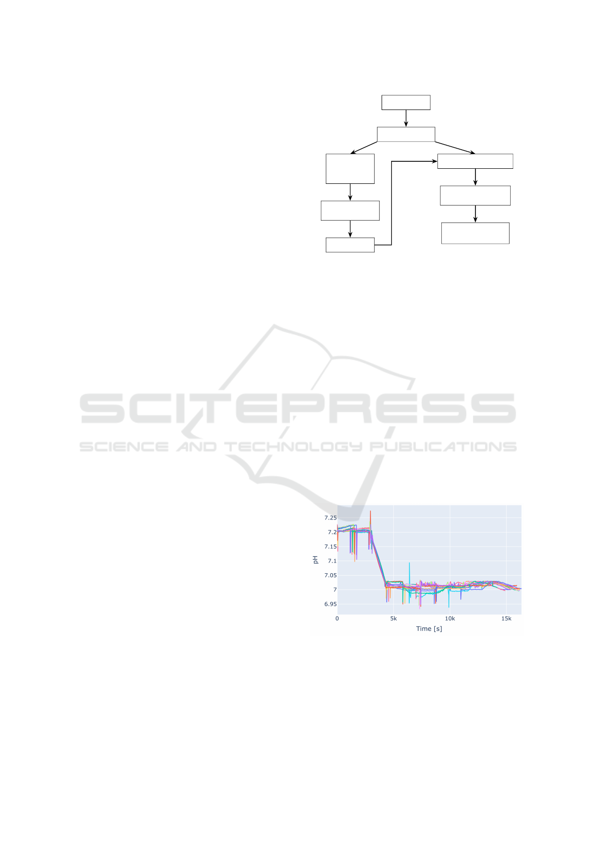
Figure 1). The framework starts with raw data, which

is initially standardized using a scaling method. The

data then proceeds through two training phases: one

for the LSTM regression model and another for the

LSTM-AE. For the regression model, data is format-

ted with past and future steps to accurately forecast

sequences of points. For the AE, the reconstructed

output is subsequently evaluated against a threshold

to detect anomalies.

3.1 Data Architecture

The dataset for this study comes from a GSK man-

ufacturing process that produces proteins for a bio-

logic drug. In this process, protein cells are culti-

vated in large bioreactors under precisely controlled

Raw Data

Standard Scaling

Input and

Output Step

Setup

Reconstruction via AE

Prediction

via LSTM model

Forecasting

Reconstruction Error

Evaluation

Anomaly Detection

via rolling threshold

Figure 1: Data ﬂow of both prediction and reconstruction

phases.

conditions—such as pressure, pH, and oxygen lev-

els—to ensure optimal cell growth. Once the cells

produce sufﬁcient proteins, they are extracted, puri-

ﬁed through a series of ﬁltration and chromatogra-

phy steps to eliminate impurities, and then rigorously

tested for quality and safety. Each variable must oper-

ate within its designated Normal Operating Condition

(NOC) to maintain the process’s integrity. A prelim-

inary variable selection, conducted by the company,

has identiﬁed critical process variables—referred to

as dynamic variables—for monitoring. These include

measurements from pH sensor and controller, Dis-

solved Oxygen sensor and controller, Vessel Weight,

Vessel Pressure, and levels of Air, CO

, O

, and N

making a total of 10 key variables. Given the multi-

variate analysis and prediction, the pH signal (shown

in Figure 2) was chosen as the reference signal since

it exhibits the highest variance among all signals.

Figure 2: Representation of pH sensor readings across dif-

ferent batches, with varying signal durations.

The data is structured in batches, with each batch

representing a distinct production cycle and captur-

ing time series data from multiple sensors, with sam-

pling period equal to 5 minutes. Although each

Enhancing Pharmaceutical Batch Processes Monitoring with Predictive LSTM-Based Framework

batch follows a similar pattern, subtle variations ex-

ist, requiring the model to detect anomalies by dis-

cerning these differences. The dataset comprises 14

training batches and 6 test batches, all adhering to

the process’s NOCs. As noted earlier, each batch

terminates upon reaching the required protein quan-

tity, resulting in variable batch lengths. Aligning

these batches is challenging, often requiring the in-

troduction of artiﬁcial sequences of points to stan-

dardize the lengths. However, this process can dis-

tort the original data distribution, introducing more

noise or misleading patterns that may compromise

the model’s ability to learn meaningful representa-

tions and, ultimately, reduce the reliability of anomaly

detection. To address this issue, we can employ an

unfolding technique commonly used in PCA appli-

cations (Lee et al., 2004). This approach transforms

a 3D data matrix (batches I × time steps K × vari-

ables J) into a 2D matrix ([batches I × time steps K]

× variables J), preserving the temporal dependencies

within each batch while enabling cross-batch anal-

ysis to detect trends or anomalies. By using this

method, the model can effectively process both tem-

poral and batch-level patterns, thus enhancing pat-

tern recognition and anomaly detection. As illustrated

in Figure 3, batch-wise unfolding—where variable

differences between consecutive time steps are ana-

lyzed—can only be applied to batches of equal length.

In contrast, variable-wise unfolding highlights inter-

batch patterns, helping to preserve and reveal devia-

tions across batches.

Batch

Variables

Time

Variable-wise

unfolding

Variables

Batch-wise

unfolding

Variables

Figure 3: Unfolding approaches for batch processes.

3.2 Data Preprocessing

To avoid an unbalanced training phase, appropriate

data preprocessing is required. In this work, the

only required preprocessing step is feature scaling

using StandardScaler, as the dataset already con-

sists of pre-selected critical process sensors, ensur-

ing that only the most relevant features are included.

StandardScaler standardizes the data by subtract-

ing the mean and scaling to unit variance, placing all

features on a comparable scale. The transformation is

deﬁned as:

z =

x −µ

(1)

where x represents the original feature signal, µ is the

mean, and σ is the variance. This standardization

prevents features with different scales or units from

disproportionately inﬂuencing the model, thereby im-

proving training convergence and enhancing result in-

terpretability (Ahsan et al., 2021).

3.3 AutoEncoder (AE)

The AE is an unsupervised, feed-forward neural net-

work that consists of two main components: an en-

coder and a decoder. The encoder compresses high-

dimensional input data into a lower-dimensional la-

tent space, effectively extracting the most relevant in-

formation. The decoder then reconstructs the original

data from this compact representation, yielding a sim-

ilar version of the input data. The model is trained to

minimize reconstruction error, which serves as a mea-

sure of data ﬁdelity. Additionally, the size of the latent

space plays a crucial role in the performance of AEs,

as more aggressive compression can lead to a greater

loss of information.

During the anomaly detection phase, the AE eval-

uates both actual and predicted data points. It con-

tinuously monitors reconstruction errors: deviations

that exceed an established threshold are ﬂagged as

potential anomalies. Figure 4 illustrates the proposed

model implementation, with the hidden layers and ac-

tivation functions deﬁned following the optimization

phase (detailed in Section 3.5). Figure 5 demonstrates

that the model accurately reconstructs the original sig-

nals with overall minimal reconstruction error. How-

ever, the error increases in regions where the model

struggles to capture rapid variations—such as infre-

quent peaks or spikes— or sequence variations that

were not common in the training batches.

3.4 Long Short-Term Memory (LSTM)

Regression Model

LSTM networks are a specialized type of RNN well-

suited for modeling sequence data, including time-

series. They are designed to overcome the vanishing

and exploding gradient problems in traditional RNNs

(Noh, 2021), enabling the learning of long-range tem-

poral patterns. As a result, LSTMs have become one

ICINCO 2025 - 22nd International Conference on Informatics in Control, Automation and Robotics

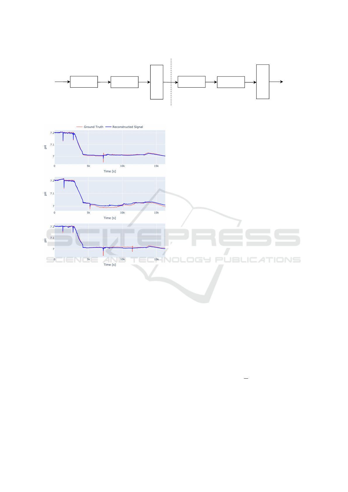
Dense

Output (1, J)

Encoder

Decoder

LSTM Layer

Units: 176

Activation Function: tanh

Dropout rate: 10%

Units: 88

Activation Function: tanh

Dropout rate: 10%

Dense

LSTM Layer

Units: 44

Activation Function: tanh

Dropout rate: 10%

Units: 176

Activation Function: tanh

Dropout rate: 10%

Latent dim: 48

Figure 4: Autoencoder structure.

Figure 5: Comparison of AE’s reconstruction ability of dif-

ferent pH signals.

of the most popular and effective RNN architecture

for time-series forecasting (Torres et al., 2021). Nu-

merous studies have adopted LSTM-based models to

predict time-dependent data, demonstrating robust re-

sults across diverse application domains (Kong et al.,

2024).

In our framework, the dataset is also fed into the

LSTM model. With its inherent capability to capture

long-term dependencies, the model learns a mapping

from sequences of past observations (inputs) to a con-

tinuous target variable (output). Traditional ML mod-

els often do not support multi-output prediction, since

they are optimized and designed for one-target case.

Input and output lags can be particularly beneﬁcial

for batch processes, where understanding both recent

changes and long-term trends is critical for monitor-

ing and control.

3.5 Parameter Optimization

The performance of Neural Network (NN) models

hinges on their architecture and hyperparameters. To

ﬁnd the best optimal set of parameters, HyperParam-

eter Optimization (HPO) is essential. Bayesan Op-

timization (BO) is a Sequential Model-Based Opti-

mization (SMBO) technique well-suited for tuning

expensive black-box functions, such as those encoun-

tered in DL. In BO, a surrogate model—often a

Gaussian Process (GP)—is used to approximate the

true objective function. Since evaluating the objec-

tive function (for instance, training an ML model) is

resource-intensive, the surrogate model signiﬁcantly

reduces computational costs by providing an efﬁcient

estimation. BO excels in exploring complex, high-

dimensional parameter spaces by effectively balanc-

ing exploration and exploitation (Wu et al., 2019).

These beneﬁts are particularly evident when com-

pared to traditional methods like grid search and

random search. Grid search becomes computation-

ally prohibitive as the number of hyperparameters

increases due to exponential growth in evaluations,

while random search can inefﬁciently allocate re-

sources by sampling suboptimal regions without fo-

cusing on promising conﬁgurations. The reconstruc-

tion capability of the AE and the prediction accuracy

of the LSTM model are optimized using BO, using

GP as the surrogate model. The objective is to mini-

mize the Mean Squared Error (MSE) between the in-

put data and the target output—the AE strives to re-

produce the input data accurately and the LSTM aims

at forecasting future data points effectively. Formally,

the optimization problem is deﬁned as follows:

⋆

= arg min

f (θ) (2)

f (θ) = MSE =

∑

i=1

∥x

− ˆx

∥

(3)

where: f (θ) is the objective function to be minimized;

θ is the hyperparameter conﬁguration vector; x

and

ˆx

represent the ground truth and reconstructed val-

ues for each sample i; and N is the total number of

samples (with each sample corresponding to a set of

Enhancing Pharmaceutical Batch Processes Monitoring with Predictive LSTM-Based Framework

sensor readings). The optimal conﬁguration θ

⋆

is the

one that yields the lowest observed objective value.

To approximate the objective function, the following

GP surrogate model is employed:

(θ) ∼ GP



m(θ), k(θ,θ

′

)



(4)

where: n is the current optimization; m(θ) = 0 (nor-

malized data) is the mean function; and the covariance

function is deﬁned as:

k(θ, θ

′

) = σ

1 +

√

ℓ

3ℓ

exp

−

√

ℓ

(5)

where: r = ∥θ −θ

′

∥; v > 0 is the smoothness param-

eter (normally v = 2.5); ℓ is the length-scale param-

eter, which scales the Euclidean distance r; and σ is

the variance. Once the surrogate model provides an

estimate, a new set of hyperparameters is chosen to

further minimize the objective function. This selec-

tion is guided by an acquisition function, typically the

Expected Improvement (EI) function, deﬁned as:

EI(θ) = E



max



0, f

best

−

(θ)



(6)

where f

best

≜ min

i=1,...,n

f (θ

) is the best observed value

of the objective function up to the current iteration. In

this study, the following hyperparameters were opti-

mized, with the MSE as the loss function.

• Model Depth: determines the number of layers

of the model.

• Units per Layer: speciﬁes the number of neurons

in each layer.

• Activation Function: deﬁnes the transformation

applied at each layer.

• Learning Rate: sets the step size for the opti-

mization algorithm.

• Latent Dimension: speciﬁes the number of neu-

rons in the encoder’s ﬁnal layer, deﬁning the size

of the latent space into which the input is mapped.

The optimal hyperparameter conﬁguration for the

training dataset is presented in Figure 4, with learning

rate equal to 8.6e

−4

. This conﬁguration enables the

AE to achieve efﬁcient performance as described in

Section 4.2.

3.6 Threshold Computation

In unsupervised anomaly detection models (e.g., au-

toencoders), selecting an appropriate threshold for the

reconstruction error is critical to distinguish normal

variations from true anomalies. One straightforward

strategy is to deﬁne the anomaly cutoff at a high

percentile of the reconstruction error distribution ob-

tained from training data. This approach ensures that

only a small fraction (e.g., 1%) of normal data would

be mistakenly classiﬁed as anomalies by design. This

should prioritize catching extreme outliers while lim-

iting false alarms (Sabzehi and Rollins, 2024). For

multivariate anomaly scoring (or when considering

the vector of reconstruction errors across multiple fea-

tures), thresholding can be based on the Mahalanobis

Distance (MD) (Ghorbani, 2019). The MD measures

how far a point is from the center of a distribution

while accounting for the covariance structure of the

data. The Mahalanobis thresholding approach has the

advantage of capturing correlations among variables

(or error components), making it more sensitive to

unusual combinations of feature values that univari-

ate methods might miss. However, it assumes a rea-

sonably well-estimated covariance matrix; in high di-

mensions or with limited data, robust covariance esti-

mation or dimensionality reduction may be necessary

to apply this method effectively.

In this study, we employ an adaptive threshold

technique based on rolling median and MAD of the

reconstruction error. The rolling median serves as a

local baseline of “normal” behavior, while the rolling

MAD provides a scale of typical variability in that pe-

riod. We then ﬂag a data point as anomalous if its

reconstruction error deviates from the current median

by more than a chosen factor times the MAD. In other

words, the threshold at time t is deﬁned as:

= median{x

| j ∈W (t)}

MAD

= median{|x

−M

| | j ∈W (t)}

= M

+ k ×MAD

(7)

where: W (t) denotes the set of indices within the

rolling window at time t; and k is a scaling factor

that adjusts the threshold to suit the dataset’s speciﬁc

requirements. This rolling median/MAD approach

yields a time-varying threshold that can adapt to grad-

ual shifts or trends in the data while still being resis-

tant to short-term spikes. It provides a simple, non-

parametric way to detect deviations that are extremes

with respect to local normal variations by carefully

setting the scaling factor and the window size based

on data distribution. For our dataset: k is set to 10 to

catch anomalies that are not mistaken for new normal

observations, caused by frequent spikes in the train-

ing data, which may lead to increased reconstruction

error; and the length of W equal to 30 to account for

local variations.

ICINCO 2025 - 22nd International Conference on Informatics in Control, Automation and Robotics

3.7 Evaluation Metrics

To evaluate the performance of the proposed model,

we utilize the following two metrics.

• Mean Squared Error (MSE): mainly used in the

optimization and training phase, it measures the

average squared difference between the predicted

values ( ˆy

) and the true values (y

). It can be ex-

pressed as:

MSE =

∑

i=1

− ˆy

)

(8)

where N is the number of samples.

• Area Under the Curve Receiver Operating

Characteristic (AUCROC): it represents the

model’s ability to distinguish between positive

and negative classes. The ROC curve plots the

True Positive Rate (TPR) against the False Posi-

tive Rate (FPR) at various thresholds. The AUC

is calculated as:

AUC =

TPRd(FPR) (9)

where:

TPR =

TP + FN

(True Positive Rate)

FPR =

FP + TN

(False Positive Rate)

(10)

The AUCROC is a single scalar value ranging

from 0 to 1, where 1 indicates a perfect distinc-

tion between normal and anomaly points.

These metrics, together, provide a comprehensive

evaluation of the model’s accuracy and its ability to

explain the variance in the data, as shown in Sec-

tion 4.1.

4 RESULTS

In order to provide an overall performance compar-

ison between our proposed AE and both traditional

and recent approaches, we leverage ADBench (Han

et al., 2022), a comprehensive public benchmark for

anomaly detection. ADBench evaluates the perfor-

mance of 30 anomaly detection algorithms, of which

14 are unsupervised, across 57 datasets, encompass-

ing a wide variety of real-world and synthetic scenar-

ios. In this benchmark, anomalies are simulated via

four distinct mechanisms: (I) local anomalies, which

deviate from the patterns of their immediate neigh-

borhoods; (II) global anomalies, generated by sam-

pling from a uniform distribution; (III) dependency

anomalies, where the natural correlations among in-

put features are deliberately disrupted; and (IV) clus-

tered anomalies, in which anomalous points occur in

concentrated groups. This setup allows for a thorough

evaluation of model performance under diverse condi-

tions, offering valuable insights of anomaly detection

capabilities.

4.1 Anomaly Detection with Generic

Dataset

As illustrated in Table 1, the average AUCROC

scores for various unsupervised models—evaluated

on datasets characterized by distinct anomaly

types—demonstrate that our approach consistently

delivers robust results even without specialized tun-

ing. Moreover, further performance improvements

are expected following HPO. For instance, while

models like KNN excel at detecting independent

anomalies and PCA proves effective for clustered

anomalies, both may struggle when confronted with

complex, interrelated anomaly patterns.

4.2 Anomaly Detection with GSK

Dataset

To assess ADBench’s models using our dataset, syn-

thetic anomalies must be incorporated into the test set

since the original data contains no outliers and can-

not be directly imported into the benchmark without

anomalies. Speciﬁcally, for each synthetic anomaly,

we randomly select one feature and one time step,

and inject anomalies corresponding to 1% of the test

data size. At the chosen time step, a spike is in-

troduced—its magnitude is determined by the data’s

standard deviation and scaled by a predeﬁned deteri-

oration factor. Table 2 shows AUCROC score of each

model with the custom dataset.

4.3 Batch Prediction & Reconstruction

Based on the data ﬂow depicted in Figure 1, data

points are analyzed in two distinct approaches: (I)

prediction followed by detection, and (II) real-time

detection. For prediction, the window corresponding

to each input lag is fed into the LSTM model, which

then produces the subsequent outputs, deﬁned by the

output lag. To analyze various combinations of input

and output values, a grid search is performed over a

range of potential input-output lag pairs, depending

on the sampling time of 5 minutes. For each pair, a

BO optimization is carried out to facilitate a compar-

ative evaluation of the results. By looking at Table 3,

Enhancing Pharmaceutical Batch Processes Monitoring with Predictive LSTM-Based Framework

Table 1: Average AUCROC evaluated on 57 datasets across ﬁve anomaly types: Default, Local, Global, Dependency, and

Cluster. For each type of anomaly, the best value is highlighted.

Model

Type of Anomaly

Original Local Global Dependency Cluster

IForest 0.7349 0.8859 0.9973 0.7820 0.9680

OCSVM 0.6922 0.8618 0.9871 0.6238 0.9569

CBLOF 0.7396 0.8918 0.9970 0.8357 0.8769

COF 0.6437 0.9065 0.9493 0.8877 0.5211

COPOD 0.7177 0.8557 0.9907 0.6065 0.9681

ECOD 0.7187 0.8785 0.9908 0.5950 0.9447

HBOS 0.7122 0.8527 0.9931 0.5982 0.9668

KNN 0.7058 0.9117 0.9991 0.8959 0.8339

LOF 0.6384 0.9359 0.9189 0.8814 0.4446

PCA 0.7194 0.8662 0.9933 0.6288 0.9782

SOD 0.6880 0.8703 0.9889 0.8940 0.7526

DeepSVDD 0.5612 0.6142 0.7507 0.6133 0.5652

DAGMM 0.6277 0.7927 0.9164 0.6526 0.9354

Proposed AE 0.7242 0.8968 0.9867 0.8984 0.8586

Table 2: AUCROC score with GSK batch dataset.

Method AUCROC

IForest 0.7555

OCSVM 0.6957

CBLOF 0.9107

COF 0.9581

COPOD 0.6721

ECOD 0.6985

HBOS 0.6643

KNN 0.9766

LOF 0.9772

PCA 0.6702

SOD 0.8932

DeepSVDD 0.6297

DAGMM 0.6570

Proposed AE 0.9844

it is evident that the error increases as the output lag

grows with a ﬁxed input lag, caused by the increas-

ing number of predictions and inherently difﬁculty of

multi-point prediction. Although extending the input

history does not linearly enhance the model’s learn-

ing capacity, our ﬁndings indicate that a 30-minute in-

put history (six data points) is sufﬁcient to forecast 15

minutes ahead (three data points). In contrast, predict-

ing 1 hour (twelve data points) accurately requires an

input history of 1 hour and 30 minutes (eighteen data

points). Figure 6 demonstrates that accuracy drops as

additional outputs are predicted, with a notable drop

in performance after 30 minutes, after which the pre-

dictions tend to become stationary. Moreover, Fig-

ure 7 shows the reconstructed pH signal from a 5-

minute prediction step along with its threshold eval-

uation. Notably, the average AUCROC across the test

set with synthetic anomalies is 0.8040, 0.5541, and

0.5507 for the rolling threshold, percentile, and MD

methods, respectively.

Table 3: Batch prediction MSE on test data based on input

and output lags.

Output Predictions

1 3 6 12

Input

Lag

6 0.0036 0.0061 0.0099 0.0209

12 0.0033 0.0067 0.0098 0.0211

18 0.0033 0.0063 0.0094 0.0191

24 0.0033 0.0075 0.0089 0.0203

5 CONCLUSIONS

In this study, we introduced an anomaly detection

approach that leverages an LSTM-AE for real-time

monitoring in batch processes. The proposed frame-

work addresses the challenges of non-linear dynam-

ics, high dimensionality, and temporal dependencies

by using reconstruction error-based detection with a

rolling threshold. This method robustly preserves es-

sential information while reducing false positives and

detecting gradual deterioration. Validated in real-

world scenarios, the LSTM-AE shows promise as

an alternative to traditional and ML approaches for

identifying subtle, complex anomalies in industrial

batch processes. Furthermore, a NN model, based

on LSTM layers, is integrated to forecast future data

points by analyzing both historical trends and antic-

ipated future steps, providing an accurate prediction

of at least 15 minutes ahead. The predictions are then

fed into the LSTM-AE, further enhancing its abil-

ICINCO 2025 - 22nd International Conference on Informatics in Control, Automation and Robotics

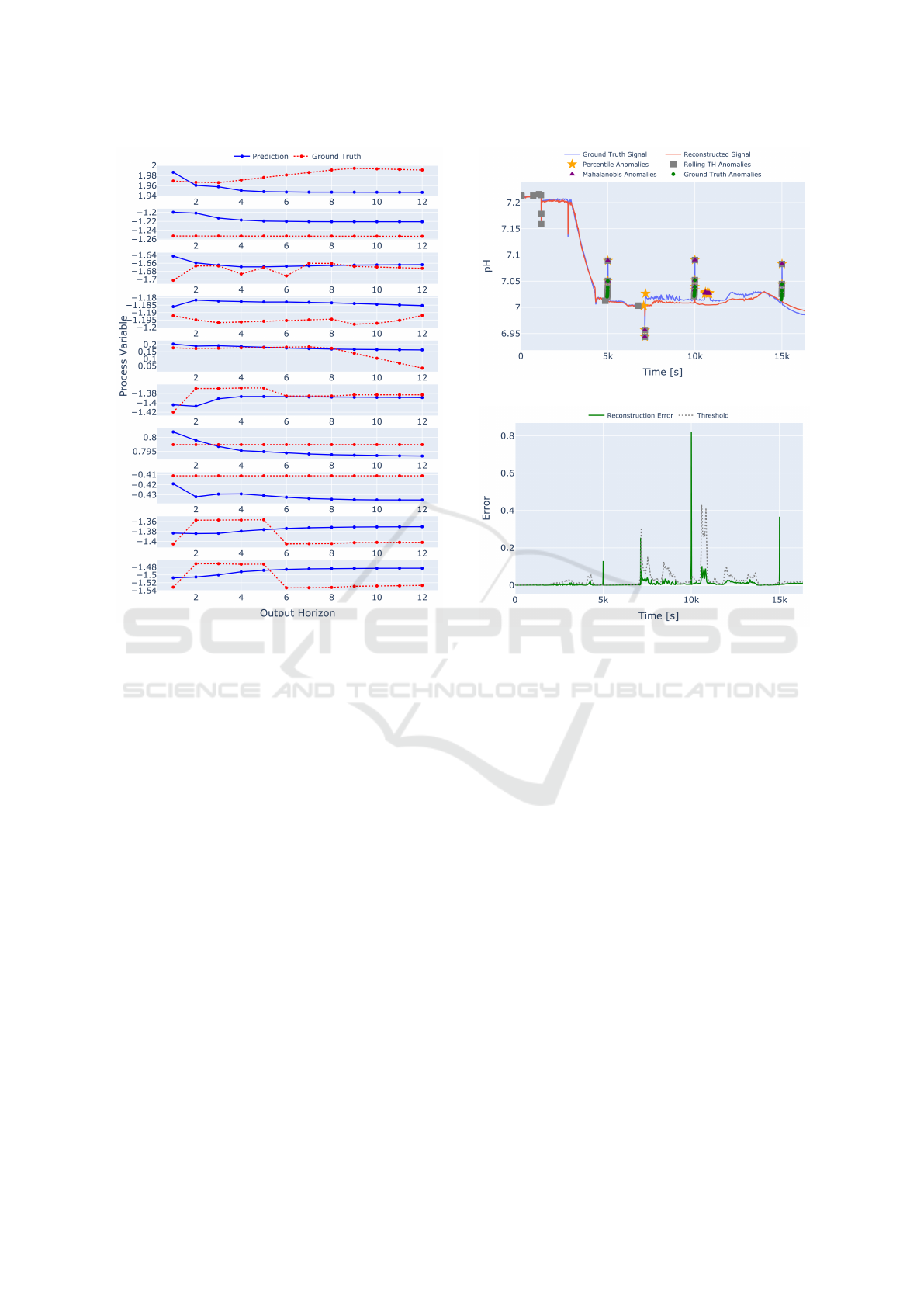
Figure 6: Predicted variables across 12 output steps (1 hour)

with 1 hour and 30 minutes of input history.

ity to anticipate deviations. This work underscores

the potential of DL techniques to revolutionize pro-

cess monitoring and anomaly detection with advanced

predictive capabilities. Future research could explore

latent space analysis for improved anomaly predic-

tion, incremental learning with real-time data, and

broader deployment across various processes by an-

alyzing critical process variables. Finally, this frame-

work may offer valuable insights in real-time indus-

trial environments into its operational efﬁciency and

scalability, especially when real faults or anomalies

are provided to increase model’s knowledge, tweak-

ing the threshold accordingly.

ACKNOWLEDGEMENTS

This work is based on a project funded by: (I) the

European Union – Next Generation Eu - under the

National Recovery and Resilience Plan (NRRP), Mis-

sion 4 Component 2 Investment 3.3 - Decree No. 352

(09th April 2022) of Italian Ministry of University

and Research - Concession Decree No. 2153 (28th

December 2022) of the Italian Ministry of Univer-

(a)

(b)

Figure 7: (a) Comparison of selected threshold mecha-

nism between predicted pH signal and its reconstruction

with synthetic anomalies; (b) reconstruction error with the

rolling threshold.

sity and Research, Project code D93D22001390001,

within the Italian National Program PhD Programme

in Autonomous Systems (DAuSy); and (II) Glaxo-

SmithKline Manufacturing S.p.a.

CONFLICT OF INTEREST

Two of the authors are employees of the GSK group

of companies. This was undertaken at the request of

and sponsored by GlaxoSmithKline Biologicals SA.

The remaining authors declare that they have no com-

peting interests.

REFERENCES

Aghaee, M., Mishra, A., Krau, S., Tamer, I. M., and Bud-

man, H. (2024). Artiﬁcial intelligence applications for

fault detection and diagnosis in pharmaceutical bio-

processes: a review. Current Opinion in Chemical

Engineering, 44:101025.

Enhancing Pharmaceutical Batch Processes Monitoring with Predictive LSTM-Based Framework

Ahsan, M. M., Mahmud, M. P., Saha, P. K., Gupta, K. D.,

and Siddique, Z. (2021). Effect of data scaling meth-

ods on machine learning algorithms and model perfor-

mance. Technologies, 9(3):52.

Choi, S. W., Lee, C., Lee, J.-M., Park, J. H., and Lee, I.-B.

(2005). Fault detection and identiﬁcation of nonlin-

ear processes based on kernel pca. Chemometrics and

intelligent laboratory systems, 75(1):55–67.

Ghorbani, H. (2019). Mahalanobis distance and its applica-

tion for detecting multivariate outliers. Facta Univer-

sitatis, Series: Mathematics and Informatics, pages

583–595.

Greenacre, M., Groenen, P. J., Hastie, T., d’Enza, A. I.,

Markos, A., and Tuzhilina, E. (2022). Principal com-

ponent analysis. Nature Reviews Methods Primers,

2(1):100.

Han, S., Hu, X., Huang, H., Jiang, M., and Zhao, Y. (2022).

Adbench: Anomaly detection benchmark. Advances

in neural information processing systems, 35:32142–

32159.

Inoue, J., Yamagata, Y., Chen, Y., Poskitt, C. M., and Sun,

J. (2017). Anomaly detection for a water treatment

system using unsupervised machine learning. In 2017

IEEE international conference on data mining work-

shops (ICDMW), pages 1058–1065. IEEE.

Jeffy, F., Gugaliya, J. K., and Kariwala, V. (2018). Ap-

plication of multi-way principal component analysis

on batch data. In 2018 UKACC 12th International

Conference on Control (CONTROL), pages 414–419.

IEEE.

Kilickaya, S., Ahishali, M., Celebioglu, C., Sohrab, F.,

Eren, L., Ince, T., Askar, M., and Gabbouj, M.

(2024). Audio-based anomaly detection in industrial

machines using deep one-class support vector data de-

scription. arXiv preprint arXiv:2412.10792.

Kong, Y., Wang, Z., Nie, Y., Zhou, T., Zohren, S., Liang,

Y., Sun, P., and Wen, Q. (2024). Unlocking the power

of lstm for long term time series forecasting. arXiv

preprint arXiv:2408.10006.

Lee, J.-M., Yoo, C., and Lee, I.-B. (2004). Fault detection of

batch processes using multiway kernel principal com-

ponent analysis. Computers & chemical engineering,

28(9):1837–1847.

Li, K.-L., Huang, H.-K., Tian, S.-F., and Xu, W. (2003).

Improving one-class svm for anomaly detection. In

Proceedings of the 2003 international conference on

machine learning and cybernetics (IEEE Cat. No.

03EX693), volume 5, pages 3077–3081. IEEE.

Liu, M., Zhu, T., Ye, J., Meng, Q., Sun, L., and Du, B.

(2023). Spatio-temporal autoencoder for trafﬁc ﬂow

prediction. IEEE Transactions on Intelligent Trans-

portation Systems, 24(5):5516–5526.

Majozi, T. (2009). Introduction to batch chemical pro-

cesses. Batch Chemical Process Integration: Anal-

ysis, Synthesis and Optimization, page 1–11.

Mockus, L., Peterson, J. J., Lainez, J. M., and Reklaitis,

G. V. (2015). Batch-to-batch variation: a key com-

ponent for modeling chemical manufacturing pro-

cesses. Organic Process Research & Development,

19(8):908–914.

Nguyen, H. D., Tran, K. P., Thomassey, S., and Hamad,

M. (2021). Forecasting and anomaly detection ap-

proaches using lstm and lstm autoencoder techniques

with the applications in supply chain management.

International Journal of Information Management,

57:102282.

Noh, S.-H. (2021). Analysis of gradient vanishing of

rnns and performance comparison. Information,

12(11):442.

Pirouz, D. M. (2006). An overview of partial least squares.

Available at SSRN 1631359.

Russell, E. L., Chiang, L. H., and Braatz, R. D. (2000).

Fault detection in industrial processes using canon-

ical variate analysis and dynamic principal compo-

nent analysis. Chemometrics and intelligent labora-

tory systems, 51(1):81–93.

Sabzehi, M. and Rollins, P. (2024). Enhancing rover mobil-

ity monitoring: Autoencoder-driven anomaly detec-

tion for curiosity. In 2024 IEEE Aerospace Confer-

ence, pages 1–7. IEEE.

Said Elsayed, M., Le-Khac, N.-A., Dev, S., and Jurcut,

A. D. (2020). Network anomaly detection using lstm

based autoencoder. In Proceedings of the 16th ACM

symposium on QoS and security for wireless and mo-

bile networks, pages 37–45.

Sakurada, M. and Yairi, T. (2014). Anomaly detection

using autoencoders with nonlinear dimensionality re-

duction. In Proceedings of the MLSDA 2014 2nd

workshop on machine learning for sensory data anal-

ysis, pages 4–11.

Sch

olkopf, B., Smola, A., and M

uller, K.-R. (1997). Kernel

principal component analysis. In International con-

ference on artiﬁcial neural networks, pages 583–588.

Springer.

Torres, J. F., Hadjout, D., Sebaa, A., Mart

ınez-

Alvarez, F.,

and Troncoso, A. (2021). Deep learning for time se-

ries forecasting: a survey. Big data, 9(1):3–21.

Wu, J. et al. (2019). Hyperparameter Optimization for Ma-

chine Learning Models Based on Bayesian Optimiza-

tion. Journal of Electronic Science and Technology,

17(1):26–40.

Zeng, L., Long, W., and Li, Y. (2019). A novel method for

gas turbine condition monitoring based on kpca and

analysis of statistics t2 and spe. Processes, 7(3):124.

Zhao, Y., Wang, S., and Xiao, F. (2013). Pattern

recognition-based chillers fault detection method us-

ing support vector data description (svdd). Applied

Energy, 112:1041–1048.

ICINCO 2025 - 22nd International Conference on Informatics in Control, Automation and Robotics