Generating Aerial Flood Prediction Imagery with Generative

Adversarial Networks

Natasha Randall

1 a

, Gernot Heisenberg

1 b

and Juan Luis Ramirez Duval

2 c

Institute of Information Science, Technical University of Applied Sciences Cologne, Germany

Institute for Natural Resources Technology and Management, Technical University of Applied Sciences Cologne, Germany

ﬁ

Keywords:

Flood Forecasting, Generative Adversarial Networks, Image Generation, Deep Learning.

Abstract:

Floods are one of the most dangerous, impactful natural disasters, and ﬂood forecasting is a critical component

of effective pre-ﬂooding preparedness. In this paper a data-driven approach to ﬂood forecasting is presented,

which provides photorealistic predictions that are less computationally expensive to generate than traditional

physically-based models. A ‘PairedAttention’ generative adversarial network (GAN) was developed, that

combines attention and content mask subnetworks, and was trained on paired sets of pre- and post-ﬂooding

aerial satellite images aligned with topographical data. The PairedAttention GAN achieved 88% accuracy and

an F1 score of 0.8 at ﬂood predictions on three USA ﬂood events, and an ablation study determined that the

digital elevation model was the most signiﬁcant factor to improving the GAN’s performance. Although the

model is a successful proof-of-concept for the effectiveness of a data-driven GAN to generate photorealistic,

accurate aerial ﬂood prediction imagery, it nevertheless struggled with generalisation, indicating an important

avenue for future research.

1 INTRODUCTION

Floods are an extremely deadly and costly natural

hazard, accounting for 47% of all weather-related dis-

asters between 1995 and 2015, leading to immense

economic damages and losses of life (CRED, 2015).

Climate change is also increasing the prevalence and

intensity of storm and ﬂooding events (UNDP, 2023).

Developing effective ﬂood risk management strate-

gies is thus more important than ever, and ﬂood fore-

casting is a critical component to supporting pre-

ﬂooding preparedness (Jain et al., 2018).

The traditional approach to making detailed ﬂood

inundation forecasts begins with a numerical weather

prediction (Ming et al., 2020). The precipitation fore-

cast is then input into hydrological models to create

hydrographs, which depict water level information

over time (Arduino et al., 2005). Using an external

coupling system, hydraulic or hydrodynamic models

use the inﬂow hydrographs as boundary conditions to

simulate the ﬂow of waters, by solving partial differ-

ential equations of continuity and momentum (Allaby,

https://orcid.org/0009-0008-0937-7417

https://orcid.org/0000-0002-1786-8485

https://orcid.org/0000-0003-2239-8921

2014). Although these ‘process-based’ models can

make highly detailed and accurate ﬂood inundation

predictions, they have a very high computational re-

quirement, as the prediction must be recomputed for

each new area (Henonin et al., 2013). The calibration

process of a hydrological model is also very time con-

suming, reaching hours or even days in length (Mihon

et al., 2013). Furthermore, process-based models re-

quire huge amounts of data that explicitly represent

the underlying physical characteristics of the ﬂood

(Devia et al., 2015), and in-depth knowledge and ex-

pertise is required to work with the hydrological pa-

rameters (Mosavi et al., 2018).

Alternatively, data-driven approaches to ﬂood

forecasting use deep learning, neural network based

models that learn from historical ﬂood data, to ap-

proximate the outputs of the computationally ex-

pensive hydraulic/hydrodynamic models (Guo et al.,

2021). At inference time, neural networks can make

much faster predictions than process-based models in

complex environments, as they can easily handle the

impact of factors like buildings or trees on diverting

ﬂuid ﬂow, which conversely add a lot of complexity

to the calculations of the hydraulic models (Liu et al.,

2019). Neural network based models can also be di-

rectly applied to unseen areas, whereas process-based

Randall, N., Heisenberg, G. and Duval, J. L. R.

Generating Aerial Flood Prediction Imagery with Generative Adversarial Networks.

DOI: 10.5220/0013663400004000

Paper published under CC license (CC BY-NC-ND 4.0)

In Proceedings of the 17th International Joint Conference on Knowledge Discovery, Knowledge Engineering and Knowledge Management (IC3K 2025) - Volume 1: KDIR, pages 15-27

models must always be retrained on the new topogra-

phy.

Furthermore, generative deep learning models are

also capable of creating photorealistic predictions and

visualisations of ﬂoodwaters, whereas the traditional

process-based models can output only numerical pre-

dictions. Hama et al. (2021) argue that colour-coded

ﬂood hazard maps are not engaging or intuitive, and

that alone, they are insufﬁcient to enhance situational

awareness and eliminate cognitive bias (L

utjens et al.,

2024). In contrast, realistic aerial imagery of pre-

dicted ﬂooding outcomes can help orient rescue per-

sonnel to landscape features (Sivanpillai et al., 2021)

and improve situational readiness for efﬁcient post-

ﬂooding interventions (Goswami et al., 2022). Com-

pelling ﬂood imagery also effectively raises aware-

ness of the potential impact of climate change on

individuals’ personal environments (Schmidt et al.,

2021).

The contributions of our work include the de-

velopment of a data-driven ﬂood prediction model,

which uses a generative adversarial network (GAN)

architecture to generate aerial ﬂood imagery that is

both photorealistic and accurate, by modelling the

ﬂood forecasting process. Quantitative state-of-the-

art results are limited, as related works have predomi-

nantly focused on photorealism and not predictive ac-

curacy (Luccioni et al., 2021) and require running ad-

ditional process-based numerical simulations to pro-

vide the accuracy to the data-driven model (L

utjens

et al., 2024). However, our GAN was trained on only

open observational data, using only tools distributed

under open licences, and without the use of any ex-

pensive simulations, thus demonstrating the viability

of a more accessible approach to developing ﬂood

prediction models.

The availability of datasets on which to train gen-

erative ﬂood prediction models is currently very lim-

ited, with no benchmark dataset, hence we also re-

lease the dataset developed for this paper. It includes

over 1000 pixel-aligned sets of pre-ﬂooding satellite

images, a high resolution digital elevation model, ﬂow

accumulation, distance to rivers, cartographical map,

and ground truth post-ﬂooding satellite images.

The research questions explored in this paper are:

• How accurately can GANs generate aerial ﬂood

prediction imagery?

• Which GAN architecture generates the most ac-

curate ﬂood predictions?

• Which topographic factors most improve the ac-

curacy of the ﬂood predictions?

• How accurately can the GANs generalise to new

ﬂood events and features?

2 RELATED WORK

The ﬁrst generative models that were used to create

images relied on a convolutional neural network ar-

chitecture (LeCun et al., 1998). Flood susceptibility

mapping using convolutional and autoencoder deep

learning architectures has been successfully demon-

strated by Wang et al. (2020) and Ahmadlou et al.

(2021) respectively. In these studies, a range of vari-

ables were input into the models, including altitude,

slope, land use and lithology, and the probability of

ﬂooding occurring at each pixel was subsequently

output.

The generative adversarial network (GAN) ex-

ploits the strength of neural networks as universal

function approximators (Hornik et al., 1989) to learn a

mapping from random noise to a synthetic image that

is indistinguishable from real images (Goodfellow

et al., 2014). The basic GAN consists of two networks

- a generator and a discriminator - that are trained si-

multaneously and work adversarially. The discrimi-

nator is a classiﬁer, which trains to better discriminate

between real images and the synthetic images created

by the generator, thus incentivising the generator to

train to generate more convincingly realistic synthetic

images, which are capable of ‘fooling’ the discrimina-

tor. The loss function of a GAN comprises the prob-

ability that the discriminator correctly predicts that

real images are real (logD(x)), and that synthetic im-

ages are synthetic (log(1 − D(G(z)))). It is therefore

described as a ‘minmax’ function, because the dis-

criminator wants to maximise this function, whereas

the generator wants to minimise it (Goodfellow et al.,

2014).

In 2017, Isola et al. introduced the Pix2Pix archi-

tecture for image-to-image translation, which gener-

ates images that are conditioned on an additional in-

put image. Pix2Pix therefore needs access to paired

image sets in order to train using a supervised learn-

ing approach. Hofmann and Sch

uttrumpf (2021) and

do Lago et al. (2023) utilised a conditional GAN ar-

chitecture to generate binary ﬂood predictions, by

training their models on data generated by hydrody-

namic simulations.

The CycleGAN architecture was developed to use

an unsupervised learning strategy without the need for

paired images, by utilising the concept of cycle con-

sistency. The CycleGAN model (Zhu et al., 2017)

consists of two generators and two discriminators.

The ﬁrst generator transforms a real image from do-

main X to domain Y, and the second generator takes

the generated domain Y image, and transforms it back

to domain X again. The cycle consistency loss then

evaluates whether the reconstructed synthetic domain

KDIR 2025 - 17th International Conference on Knowledge Discovery and Information Retrieval

X image correctly matches the original real domain X

image. CycleGAN’s loss function is formed from the

cycle consistency losses from both the forwards and

backwards cycles, as well as the adversarial losses

contributed by the discriminators, which assess the

realism of the synthetic images in both domains (Zhu

et al., 2017).

Rui et al. (2021) and Luccioni et al. (2021)

used GAN architectures, including the CycleGAN

(Schmidt et al., 2019), to create engaging, realistic

‘street-view’ images of ﬂoods. L

utjens et al. (2024)

and Goswami et al. (2022) focused on generating

accurate and photorealistic aerial ﬂood imagery, but

their models relied on pre-segmented labelled masks

to deﬁne the correct ﬂoodwater locations, and did not

use the GAN model to make the predictions.

Hama et al. (2021), Schmidt et al. (2021) and

Goswami et al. (2022) all concluded that training a

model on labelled ﬂood masks greatly improves the

generated images of ﬂoods. However, obtaining la-

belled data is extremely time consuming and expen-

sive. ‘Attention’ mechanisms represent an alterna-

tive approach to achieve a similar result, without the

need for the labelled mask data. AttentionGAN (Tang

et al., 2021) trains subnetworks to produce attention

masks and content (image transformation) masks; the

attention masks are then applied to the content masks,

which are then added to the original image pixel-wise,

hence only the area of the image indicated by the at-

tention mask is transformed. AttentionGAN also uses

the same unsupervised learning approach and cycle

consistency loss function as CycleGAN.

3 METHODOLOGY

3.1 Dataset

The study area consists of three ﬂood events in the

USA, caused by Hurricane Harvey in the city of

Houston in 2017, Hurricane Florence in North Car-

olina near the Northeast Cape Fear river in 2018,

and heavy rainfall in the Midwestern United States

along the Arkansas river in 2019. This set of events

comprises a variety of geographical regions, from the

countryside to urban settlements, as well as a range of

different precipitation intensities.

The selection of features for the dataset was de-

termined by the most impactful factors on the likeli-

hood of ﬂuvial (river) and pluvial (rainfall) ﬂooding

occurring in a particular area. The formal deﬁnition

of a ﬂood is “a body of water which rises to over-

ﬂow land which is not normally submerged” (Ward,

1978), hence the quantity of runoff is a function of

rainfall intensity and the inﬁltration capacity of the

ground, which in itself is modiﬁed by the characteris-

tics of the surface (Bolt et al., 2013). Also important

are the attributes of the overall catchment area, which

determines the dynamics of the water ﬂow. Key fea-

tures therefore include the shape, slope, aspect, alti-

tude, climate, geology, soil type, inﬁltration, vegeta-

tion cover, and channel factors of a region (Smith and

Ward, 1998).

To assist the model in making ﬂood predictions,

ﬁve factors were selected as model inputs. These

include a pre-ﬂooding optical satellite image, a dig-

ital elevation model (DEM), representation of ﬂow

accumulation, distance to nearby rivers, and a car-

tographical map. The data sources and attributions

are provided in section 6. Having access to high-

resolution, optical satellite imagery of the region be-

fore the ﬂood event had occurred, was essential for

the model to be able to generate photorealistic post-

ﬂooding aerial images. A DEM is critical for accurate

ﬂood forecasting, as it encapsulates key information

on topographical features such as elevation, slope, as-

pect, roughness and curvature (Mujumdar and Kumar,

2012). Land use, land cover and imperviousness data

were not directly input into the model, because the

openly available datasets were of poor resolution, and

were typically created by automated models classify-

ing satellite imagery (Kontgis, 2021), thus it was de-

termined to be feasible for the GAN to extract this

information itself from the pre-ﬂooding images. The

cartographical map input also provides some indica-

tion of land use, as well as the locations of roads

and buildings. It was also important to input into

the model data that described the wider context of the

study area; the distance to nearby rivers is a basic but

crude method to achieve this, whereas the ﬂow accu-

mulation provides a detailed deterministic prediction

of which cells drain into other downslope cells, hence

determining the catchment areas (Mark, 1983).

Optical Satellite Images: The ‘xBD’ dataset con-

tains paired satellite images captured before and after

ﬂood events, in the exact same locations. The im-

ages are taken from the Maxar Open Data program,

and were made by the GeoEye-1, WorldView-2 and

WorldView-3 satellites. Each image has 1024×1024

pixels in a three-band RGB format, with a resolution

of approximately 0.5 metres/pixel. The pre-ﬂooding

satellite image is input into the model, whereas the

paired post-ﬂooding image functions as the ground

truth target, used to evaluate the predictions made by

the model.

Digital Elevation Model: The USGS 3D Ele-

vation Program DEM, which has a 1/3 arc-second

(10 metre) resolution, describes the topography of the

Generating Aerial Flood Prediction Imagery with Generative Adversarial Networks

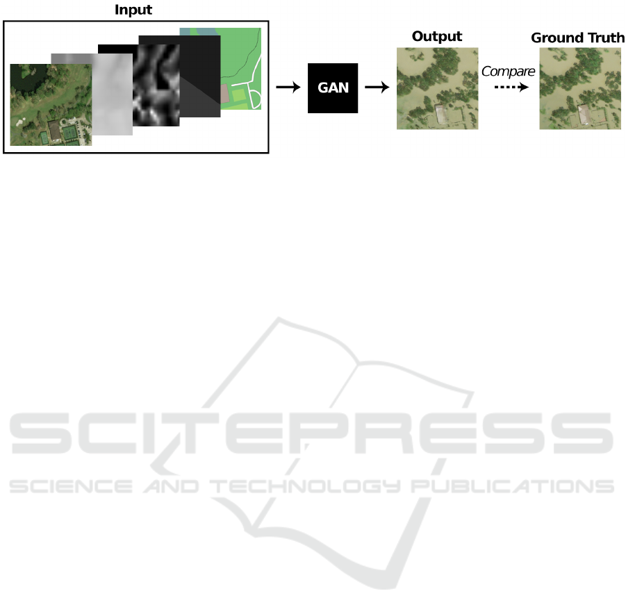
Figure 1: A single image stack comprised of a pre-ﬂooding satellite image, DEM, ﬂow accumulation, distance to rivers,

and map, is input into the GAN model. The GAN outputs a synthetic, predicted post-ﬂooding satellite image, which can be

evaluated by comparing it to the real ground truth post-ﬂooding image.

study areas. The elevations in this DEM represent the

topographic bare-earth surface, hence excluding ob-

jects like trees and buildings, which are instead repre-

sented in the pre-ﬂooding satellite images.

Flow Accumulation: We calculated the ﬂow ac-

cumulation from DEM rasters that each covered ap-

proximately 2000km

, containing a study area and its

surrounding areas. It was ﬁrstly necessary to ﬁll the

sinks, to prevent artiﬁcial depressions from trapping

water and preventing continuous ﬂow (Wang and Liu,

2006). Next, the ﬂow direction and subsequent ﬂow

accumulation was calculated using the multiple ﬂow

direction algorithm (Wolock and McCabe Jr, 1995),

in the SAGA GIS tool (Conrad et al., 2015). Rather

than applying a threshold to the output, logarithm

base 10 was taken of the ﬂow accumulation values,

in order to retain the most detail for the model.

Distance to Rivers: The QGIS software was used

to visualise buffer distances (at 0.5km intervals) to all

major rivers and waterways, as classiﬁed by the Open

Street Map.

Map: OpenStreetMap data was downloaded from

Planet OSM and processed using the Osmium tool.

The Maperitive software was then used to apply a

custom ruleset to the maps’ appearance, removing all

of the text, and enhancing the clarity of the land use

types.

Input Stack: All of the inputs were georefer-

enced, and projected to the same WGS 84 coordinate

system that the satellite images originally used. The

satellite images did not compose a continuous image

of the study area, but rather captured separate, rel-

evant locations. As such, the four input features of

the DEM, ﬂow accumulation, distance to rivers and

map (henceforth referred to collectively as the “topo-

graphical factors”) were cropped to create individual

image stacks. Figure 1 depicts how a single sample

image stack is input into the model, which then out-

puts a synthetic post-ﬂooding satellite image, that can

hence be compared to the ground truth post-ﬂooding

image. Each image set contains a single pre-ﬂooding

satellite image and its associated topographical fac-

tors concatenated as tensor channels, with each pixel

representing the same 0.5m×0.5m geographical area

in all of the channels. All of the input stacks had their

alignment manually reviewed and adjusted to correct

for any errors or skewness.

The data were transformed by resizing each

1024×1024 pixel image to 512×512 pixels using

bicubic resampling, and then cropped into 4 sepa-

rate images of 256×256 pixels each, because the

model architectures worked most optimally with ex-

actly 256×256 pixel images. Although many tech-

niques have been developed to better handle higher

resolution imagery (Karras et al., 2017), (Wang et al.,

2018), the inclusion of these would have added yet

another layer of complexity to an already highly com-

plex task. The only augmentation applied to the data

was a horizontal ﬂip; the images were not rotated or

ﬂipped vertically, as such a transformation would be

unrealistic for this domain.

The ﬁnal dataset contained a total of 5736 image

stacks, of which 2680 corresponded to Hurricane Har-

vey, 1880 image stacks of Hurricane Florence, and

1176 image stacks of the Midwest ﬂoods. The data

were split into 80% in the training dataset, 10% in the

validation set, and 10% in the test set. The splits were

stratiﬁed by the ﬂood events, so that each ﬂood was

represented proportionally in each set. All of the fol-

lowing results, metrics and sample generated images

are taken from the test dataset, which was held-out

during the model training process.

3.2 Models

Although the current state-of-the-art in generative

networks tends towards the vision transformer (Doso-

vitskiy et al., 2020) and diffusion model (Ho et al.,

2020) architectures, GANs are in comparison less

computationally intensive and require less data to

train. They are also much faster at inference time,

requiring only one forward pass, as opposed to the

KDIR 2025 - 17th International Conference on Knowledge Discovery and Information Retrieval

multiple de-noising steps of a diffusion model.

GAN architectures were therefore used to gener-

ate the aerial ﬂood prediction imagery in this work,

as they best fulﬁlled the requirement of a data-driven

model that could be faster than process-based models,

and could train efﬁciently on the comparably small

size of the ﬂood dataset. The performance of three

existing model architectures was compared; Pix2Pix,

representing the supervised approach, CycleGAN,

representing the unsupervised approach, and Atten-

tionGAN, representing the guided approach. The at-

tention mechanism in the AttentionGAN architecture

is very suited for ﬂood prediction, because the atten-

tion masks can identify the location for the ﬂooding,

and the content masks can generate ﬂoodwater visu-

alisations. However, AttentionGAN’s unsupervised

learning strategy does not make effective use of the

paired pre- and post-ﬂooding images available in the

dataset. A new model called ‘PairedAttention’ was

hence created, which utilises the architecture of At-

tentionGAN, but the supervised training approach and

loss function of Pix2Pix.

The training procedures and model architectures

were replicated from their original papers, with the

exception that all of the generators and discrimina-

tors in the CycleGAN and AttentionGAN architec-

tures were modiﬁed to input the additional topograph-

ical factors. A comprehensive hyperparameter tuning

analysis determined the following optimal hyperpa-

rameters for the models: The model weights were

initialised from a Gaussian distribution with mean 0

and standard deviation 0.02. The optimizer used the

Adam algorithm (Kingma, 2014) with a learning rate

of 0.0002 and beta decay rates of 0.5 and 0.999. The

learning rate scheduler maintained the initial learning

rate for the ﬁrst half of epochs, then reduced the learn-

ing rate linearly for the second half of epochs. Each

model trained for 200 epochs, as performance was

found to plateau beyond this point. The batch size

was set to 1.

3.3 Evaluation Metrics

Because GANs generate photorealistic imagery, eval-

uating their outputs is much more difﬁcult than eval-

uating the performance of traditional classiﬁer neu-

ral networks (Betzalel et al., 2022). Determining the

most appropriate metrics is therefore key to any eval-

uation of GANs, and is highly dependent on the char-

acteristics of the data and the goal of the research.

For the task of generating aerial ﬂood prediction im-

agery, there are three core objectives: achieving a

high level of photorealism, predictive performance,

and efﬁciency.

All three of these goals are critical to making a

good ﬂood prediction. The images must be photo-

realistic in order to create a convincing representa-

tion that is useful for enhancing situational awareness.

The photorealism metrics that were used to evaluate

the GANs are: PSNR, SSIM, MS-SSIM, and LPIPS

(Arabboev et al., 2024). These metrics compare how

close a generated image is to a reference image from

their signal-to-noise ratio, by the similarity of their

structure, luminance and contrast, on multiple resolu-

tion scales, and by their feature maps, respectively.

As well as generating photorealistic imagery, it is

also important that the GANs accurately position the

ﬂoodwaters within the generated images. The perfor-

mance metrics (MSE, accuracy, F1, precision and re-

call scores) hence evaluate the predictive power of the

models, by comparing binary ﬂood masks extracted

from both a generated image and its corresponding

ground truth post-ﬂooding image. The ﬂood masks

were produced by a trained ﬂood segmentation model,

which could identify the ﬂooded pixels in the images

with an accuracy (evaluated on a held-out test set of

ﬂood masks) of 94.9% and MSE of 0.051. Although

the additional degree of error induced by the segmen-

tation model should be taken into consideration when

assessing the absolute performance of the GANs, this

error is small, and relative comparisons can still be

dependably made.

Finally, one of the main advantages of using a

data-driven approach over traditional ﬂood forecast-

ing methods, is that it should be faster and use fewer

computational and human resources. The two mea-

surements used to evaluate the efﬁciency of the mod-

els were the training time (the total time needed to

train the model) and the inference time (the time

needed for the model to make a ﬂood prediction and

generate an image).

Nevertheless, there are limitations inherent to all

of the evaluation metrics. For example, if a ﬂood

prediction is off by simply one pixel, it would be pe-

nalised by the performance metrics, even though to a

human eye there may be no visible difference. Chlis

(2019) argues that the most reliable way to evaluate

the performance of a GAN is therefore to manually

inspect the quality of the generated images. As such,

sample images are also included throughout the pre-

sentation of the results.

Generating Aerial Flood Prediction Imagery with Generative Adversarial Networks

4 RESULTS

4.1 Model Architectures Performance

Table 1 presents the performance of the four model

architectures PairedAttention, Pix2Pix, Attention-

GAN, and CycleGAN. The two models that use a

supervised training approach (PairedAttention and

Pix2Pix) achieved better results than the two cycle-

based models (AttentionGAN and CycleGAN) on all

of the photorealism and performance metrics, with

PairedAttention performing the best overall. Fig-

ure 2 displays sample images generated by each of

the model architectures, and demonstrates that the

PairedAttention model is able to consistently generate

post-ﬂooding imagery that is not only photorealistic,

but makes accurate ﬂood predictions.

There is no strong pattern depicted in ﬁgure 3(b),

suggesting that the GAN is capable of making accu-

rate predictions at varying ﬂood amounts, from 0%

to almost 100% of the image being ﬂooded. Figure

3(c) plots the distribution of the MSE for only in-

stances where 1% or less of the ground truth image

contains ﬂooded pixels. The histogram is extremely

right skew, indicating that the model is able to cor-

rectly identify when the area depicted in an image

should have little to no ﬂooding. The models were

also able to successfully learn the key features of river

ﬂoods, including how rivers break their banks and

ﬂood adjacent low-lying areas (as in ﬁgure 2(c)).

The cycle-consistency terms in the loss functions

of the cycle-based models assisted these models in

recreating the ﬁne details in the images, such as the

clean lines of buildings. However, AttentionGAN and

CycleGAN have substantially lower recall scores than

PairedAttention and Pix2Pix, corresponding to fail-

ures to generate ﬂooding in areas of the images that

should have been ﬂooded. This error occurs because

cycle-based methods assume a one-to-one mapping

instead of a many-to-one mapping (Schmidt et al.,

2019). When the ﬁrst generator transforms many dif-

ferent features - such as roads, grass, or mud - all

into ﬂoodwaters, then the second generator is unable

to determine which feature the ﬂoodwaters should

be transformed back into, when attempting to recon-

struct the original image (Luccioni et al., 2021). In

order to improve the cycle consistency loss, the cycle-

based methods therefore tend to avoid modifying and

hiding as much of the original pre-ﬂooding image as

possible, as can be seen in ﬁgure 2(b), where Atten-

tionGAN and CycleGAN do not place ﬂoodwaters

over the lake, so that the lake can be more easily re-

constructed later.

Due to the two generators and two discriminators

required by the AttentionGAN and CycleGAN mod-

els, they also use the most computational resources to

train, whereas the PairedAttention and Pix2Pix mod-

els were trained in approximately a third of the time

(table 1). After the models have been trained just

once on the historical data however, they can be ap-

plied to any new unseen areas, all taking only approx-

imately 0.004 seconds to generate an image predic-

tion. In comparison, as reported in research compar-

ing data-driven models to traditional methods, Hof-

mann and Sch

uttrumpf’s (2021) process-based hydro-

dynamic model took 7 hours to perform a detailed

simulation, whereas Kabir et al. (2020) and do Lago

et al. (2023) required 1.3 hours and 1.5 hours to sim-

ulate a single event with a 2D hydrodynamic and hy-

draulic model respectively. The advantage of the data-

driven approach is evident, as once trained, the GANs

can be applied to a variety of previously unseen im-

ages with extremely fast inference times, whereas the

process-based models must always rerun their simu-

lations.

4.2 Impact of Topographical Factors

An ablation study was carried out in order to ascer-

tain the impact of the different topographical factors

on the performance of the GANs. Speciﬁcally, the

pre-ﬂooding satellite image was always input into the

model, (as it is a requisite to be able to generate a pho-

torealistic image), and in each experiment just one of

the topographical factors was additionally input into

the model. Table 2 presents the results from mod-

els using the PairedAttention architecture, the ﬁrst of

which utilised all of the input factors as a baseline.

The remaining models input a combination of only

the pre-ﬂooding satellite image and the DEM, or only

the satellite image and the ﬂow accumulation repre-

sentation, etc. The ﬁnal model, labelled ‘None’, was

input with the pre-ﬂooding satellite image alone.

With regards to the photorealism metrics, all of

the models performed similarly. This is not unex-

pected, as the realism of the generated post-ﬂooding

image depends predominantly on a transformation of

the pre-ﬂooding image, which was input to all of

the models. In all of the performance metrics, ‘All’

‘DEM’ and ‘Flow accumulation’ outperformed ‘Dis-

tance to rivers’ ‘Map’ and ‘None’. This result indi-

cates that the elevation values (as the ﬂow accumula-

tion was also derived from the DEM) are the most im-

portant to making accurate ﬂood predictions. This is

also evident in ﬁgures 4(a) and (b), where the models

without access to elevation information often either

under-ﬂood or over-ﬂood areas in the images. ‘Dis-

tance to rivers’ and ‘Map’ did not perform better than

KDIR 2025 - 17th International Conference on Knowledge Discovery and Information Retrieval

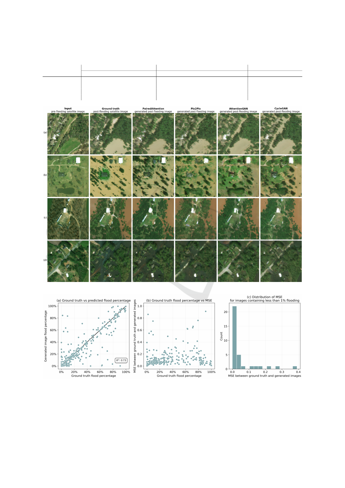
Table 1: The results from evaluating the performance of the four model architectures on predicting the ﬂood events.

Model Architectures

Photorealism Metrics Performance Metrics Efﬁciency Metrics

PSNR↑ SSIM↑ MS-SSIM↑ LPIPS↓ MSE↓ Accuracy↑ F1↑ Precision↑ Recall↑ Inference↓ (s) Training↓ (h)

PairedAttention 22.681 0.573 0.683 0.228 0.123 0.877 0.804 0.824 0.786 0.004 15.3

Pix2Pix 22.442 0.557 0.644 0.250 0.134 0.866 0.781 0.824 0.742 0.004 11.3

AttentionGAN 21.394 0.524 0.581 0.261 0.157 0.843 0.738 0.796 0.689 0.004 43.6

CycleGAN 20.841 0.510 0.578 0.269 0.156 0.844 0.735 0.808 0.673 0.004 38.1

Figure 2: Sample generated images of ﬂood events from each of the four model architectures.

Figure 3: The performance of the PairedAttention GAN at different percentages of ﬂooding amounts in the post-ﬂood images.

Generating Aerial Flood Prediction Imagery with Generative Adversarial Networks

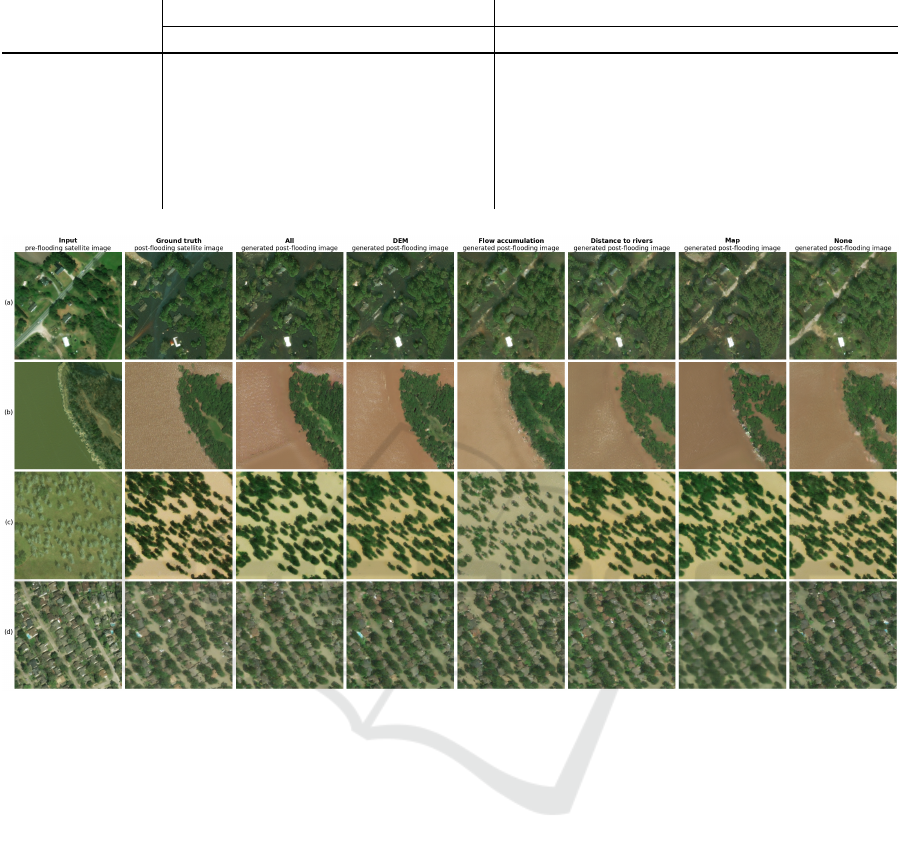
Table 2: The results from the ablation study, comparing the models using different topographical factors as inputs.

Input Topography

Photorealism Metrics Performance Metrics

PSNR↑ SSIM↑ MS-SSIM↑ LPIPS↓ MSE↓ Accuracy↑ F1↑ Precision↑ Recall↑

All 22.681 0.573 0.683 0.228 0.123 0.877 0.804 0.824 0.786

DEM 23.134 0.585 0.701 0.220 0.116 0.884 0.812 0.844 0.782

Flow accumulation 23.126 0.590 0.701 0.222 0.126 0.874 0.798 0.822 0.776

Distance to rivers 22.913 0.584 0.693 0.229 0.141 0.859 0.770 0.809 0.735

Map 22.834 0.597 0.691 0.269 0.140 0.860 0.772 0.811 0.736

None 22.900 0.583 0.690 0.231 0.140 0.860 0.772 0.812 0.736

Figure 4: Sample generated images of ﬂood events from models trained on different topographical factors. For example,

‘DEM’ means the model was input only with the pre-ﬂooding satellite image and the ‘DEM’ factor.

‘None’ - it is likely that the descriptions of land use

provided by the map can already be learned by the

model from the pre-ﬂooding satellite image, and the

‘distance to rivers’ is too simplistic of a measure in

comparison to the more detailed ﬂow accumulation.

Although access to elevation values consistently

improved the performance of the models, the absolute

differences between the metric scores is still fairly

small, and the model can achieve an accuracy of 86%

even when no topographical factors are input. There

are two explanations which could potentially account

for this result. Firstly, the model may be capable of in-

ferring more information than expected from the pre-

ﬂooding satellite image alone, including approximate

elevation values. Secondly, an investigation of the full

test dataset revealed a large number of post-ﬂooding

satellite images where simply the entire ground area

of the image is ﬂooded, (as in ﬁgures 4(c) and (d)),

and thus a detailed analysis of the topography is un-

necessary for the model to make an accurate ﬂood

prediction. Nevertheless, in more complex images for

which the topography is relevant to the positioning of

the ﬂoodwaters, having access to the elevation values

makes a signiﬁcant difference to the performance of

the model, such as in ﬁgures 4(a) and (b). However,

because the contents of the dataset instead tends to be

biased towards images like 4(c) and (d), the metrics

therefore do not properly reﬂect the importance of the

DEM.

4.3 Evaluating Model Generalisability

Although the test dataset contains images of geo-

graphical areas never before seen by the model during

training, these images are still from the same ﬂood

events that the model previously trained on. Thus

to examine the true generalisability of the GANs, a

PairedAttention model was trained on images from

Hurricane Harvey and Hurricane Florence, and eval-

uated on images of the Midwest ﬂoods. The general-

KDIR 2025 - 17th International Conference on Knowledge Discovery and Information Retrieval

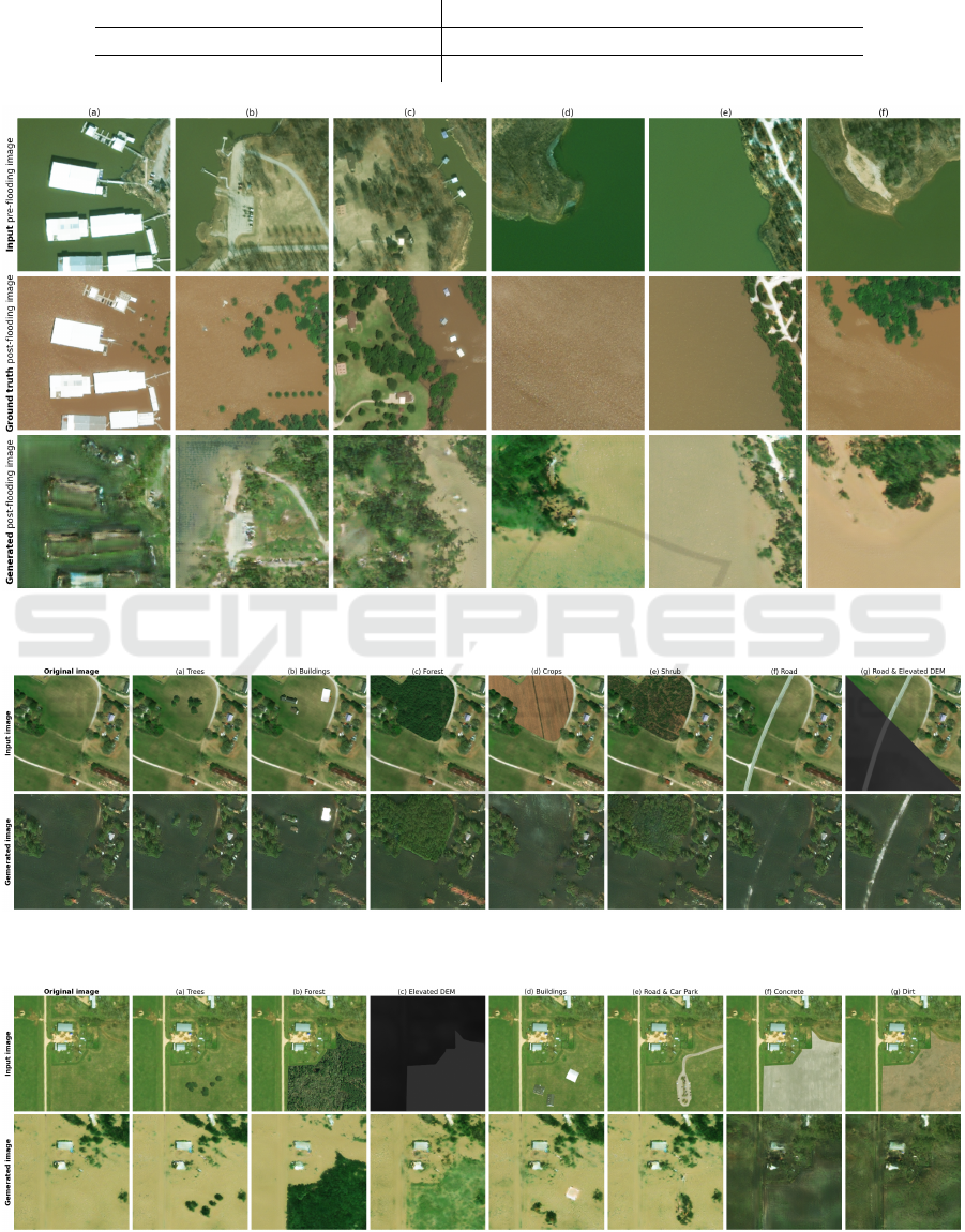
Table 3: The generalisability study results: The model was trained on data from Hurricane Harvey and Hurricane Florence,

and then evaluated on unseen data from the Midwest ﬂoods.

Photorealism Metrics Performance Metrics

PSNR↑ SSIM↑ MS-SSIM↑ LPIPS↓ MSE↓ Accuracy↑ F1↑ Precision↑ Recall↑

19.843 0.497 0.536 0.373 0.220 0.780 0.655 0.887 0.519

Figure 5: Sample generated images of the Midwest ﬂood event, produced by a model trained only on the Hurricane Harvey

and Hurricane Florence ﬂood events.

Figure 6: The changes to the generated images after different modiﬁcations have been made to a pre-ﬂooding satellite image

of the Hurricane Florence ﬂood event, such as editing in more trees (a) or increasing the elevation values of the road (g).

Figure 7: The changes to the generated images after different modiﬁcations have been made to a pre-ﬂooding satellite image

of the Hurricane Harvey ﬂood event.

Generating Aerial Flood Prediction Imagery with Generative Adversarial Networks

isability study results are presented in table 3.

The photorealism metrics are fairly poor, because

the model had not learned how to appropriately trans-

form the features and objects unique to the Midwest

ﬂoods, thus creating artifacts and blurry sections in

the generated images, as can be seen in ﬁgures 5(a),

(b) and (c). The model was also unable to predict the

correct colour of the ﬂoodwaters (dark brown) instead

replicating the yellow and blue appearances of the wa-

ters from Hurricane Harvey and Hurricane Florence.

The performance metrics also reveal the weak pre-

dictive power of the model, with an F1 score of 0.66

and a low recall score of 0.52, indicating that the

model signiﬁcantly underpredicts ﬂooding (as in ﬁg-

ure 5(d)) even though the Midwest ﬂoods experienced

less total rainfall (45-55cm) than the Hurricane Har-

vey ﬂood event that the model had trained on (75-

100cm). The representations of the core features of

each ﬂood event, such as the associated amount of

precipitation and corresponding runoff, are therefore

entangled with each of the ﬂood events. The model

has overﬁt to each ﬂood event rather than only having

learned general principles regarding the contributions

of different features to the likelihood of ﬂooding.

Nevertheless, there is evidence that the model has

learned some generalisable principles. The appear-

ance of the post-ﬂooding satellite images in ﬁgure 5

possess a modicum of coherence, with recognisable

recreations of trees, buildings and roads. The model

has also learned some of the characteristics of ﬂuvial

ﬂooding - likely from the Hurricane Florence data -

as it is able to accurately ﬂood the banks of the river

in ﬁgures 5(e) and (f).

The capability of the model to generalise to new

features in the images was also investigated, in con-

junction with an analysis of the explainability of the

model’s behaviour. Because a GAN is a black-box

model, it can be interpreted only via post-hoc meth-

ods; by changing the input to the model, and eval-

uating the subsequent change to its outputs (Ribeiro

et al., 2016). Figure 6 demonstrates how manual al-

terations to a pre-ﬂooding satellite image of Hurri-

cane Florence change the post-ﬂooding image gener-

ated by the GAN. The generated images show how

the model has not only learned to classify different

objects, but that it understands how ﬂoodwaters phys-

ically interact with each of them, ﬂowing around trees

and buildings (ﬁgures 6(a), (b) and (c)) but over crop-

land (ﬁgure 6(d)). The model also demonstrates con-

sistency, as the ﬂooding elsewhere in the image is un-

changed when an independent element of the image

is altered. In ﬁgure 6(g), the elevation of the road was

increased by modifying the values of the DEM, and

the GAN subsequently no longer ﬂoods the road, in-

dicating that it has learned the relationship between

elevation and ﬂooding. The model thus utilises fea-

tures from both the pre-ﬂooding satellite image and

the topographical factors to make ﬂood predictions.

Figure 7 depicts similar manual alterations to a

pre-ﬂooding satellite image of Hurricane Harvey. In

ﬁgures 7(a) and (b) the model is able to correctly

identify and avoid covering the trees with ﬂoodwa-

ters. Increasing the elevation values of the DEM (ﬁg-

ure 7(c)) results in the model appropriately reducing

the amount of ﬂooding within the modiﬁed area, sug-

gesting that the GAN has learned a general function

connecting elevation and ﬂoods, that is applicable to

different contexts. However, when the model encoun-

ters an unfamiliar combination of objects and settings,

such as a car park or residential housing in a rural

region, it does not know how to handle them cor-

rectly, instead transforming the objects into trees (ﬁg-

ures 7(d) and (e)). When a large surface of concrete or

dirt is added, (ﬁgures 7(f) and (g)), the model ﬂoods

the entire image with the blue ﬂoodwaters typically

associated with the Hurricane Florence ﬂood event.

This outcome suggests that the GAN does not con-

tain knowledge of impervious concrete surfaces that

is disentangled from the ﬂood events; rather the model

may use cues in the form of particular colours and tex-

tures within the image in order to determine the ﬂood

event that the image likely depicts, and accordingly

makes assumptions regarding the probable locations

and amounts of ﬂooding.

5 DISCUSSION

With regards to the research questions, the results can

be summarised:

How accurately can GANs generate aerial ﬂood

prediction imagery, and which GAN architecture

generates the most accurate ﬂood predictions? The

PairedAttention GAN architecture had the best efﬁ-

ciency, photorealism and performance metrics, with

an accuracy of 88%, F1 score of 0.80, precision of

0.82, and recall of 0.79. Overall, the supervised train-

ing approach on paired images was more effective and

trained more quickly than the cycle-based approach.

Which topographic factors most improve the

accuracy of the ﬂood predictions? The ablation

study revealed that the elevation values were the most

signiﬁcant factor for improving ﬂood predictions. Al-

though the metrics suggested that the impact of the

DEM on model performance was limited, these re-

sults were attenuated by the GAN’s capability to in-

fer information from the pre-ﬂooding satellite image

alone, as well as the dataset’s bias towards images for

KDIR 2025 - 17th International Conference on Knowledge Discovery and Information Retrieval

which the knowledge of detailed elevation values was

unnecessary to make an accurate ﬂood prediction.

How accurately can the GANs generalise to

new ﬂood events and features? Manual alterations

to pre-ﬂooding satellite images demonstrated that the

GAN model has learned how ﬂoodwaters physically

interact with different types of objects in an image,

as well as the connection between ﬂooding and el-

evation values, providing some explanation for the

model’s decisions when generating a post-ﬂooding

image. However, the model sometimes acted un-

expectedly when handling out-of-distribution inputs.

Although there were indications that the GAN had

learned some general principles regarding ﬂooding,

overall, the model performed poorly when applied to

a previously unseen ﬂood event. These results suggest

that the core features of each ﬂood event are highly

entangled within the model, rather than the model

having learned a generalisable function.

Unlike hydraulic or hydrodynamic models, a

GAN is not only learning to make ﬂood predictions,

but also to generate photorealistic imagery. The

GAN’s training process thus incorporates both adver-

sarial and L1 loss terms in the loss function, which

respectively regulate the overall photorealism of the

generated image, and the similarity of the entire im-

age to the ground truth image. Consequently, opti-

mising the accuracy of the ﬂood predictions is only a

small part of the GAN’s objective, and is a part that is

only ever learned indirectly.

This training approach also resulted in a highly en-

tangled representation of concepts within the model.

In a disentangled data representation, individual fac-

tors (such as the amount of precipitation) are iso-

lated and captured by separate, distinct elements of

the model’s representations, and hence can be var-

ied independently (Bengio et al., 2013). However

the ﬂood prediction GANs had strongly overﬁt to the

ﬂood events that they were trained on, with the ﬂood

factors inextricable from the events themselves.

Future work should therefore focus on improv-

ing the generalisability of ﬂood prediction models.

A generalisable data-driven model also ampliﬁes its

advantages over numerical process-based models, as

it can quickly generate predictions for a wider vari-

ety of areas and scenarios. The model thus needs

to learn disentangled data representations, which can

be achieved by adapting the model architecture, loss

functions and the training dataset (Wang et al., 2022).

Isolating the independent inﬂuence of factors such as

precipitation would allow the model to dynamically

condition the generated ﬂood predictions on input

weather forecasts. Due to the signiﬁcantly faster in-

ference times of data-driven models in comparison to

traditional physically-based models, a fully disentan-

gled model could even be extended to ﬂood risk man-

agement applications, by revealing how ﬂood predic-

tions change when the pre-ﬂooding input image is

modiﬁed, such as through the addition of ﬂood relief

channels or barriers (Pender and Faulkner, 2010). A

GAN model could also be utilised in conjunction with

traditional ﬂood inundation maps that reduce subjec-

tivity, with consideration of the described limitations

of the ﬂood prediction GAN, in order to avoid false

alarms during operational usage.

The performance of the GANs was evaluated by

using a separate segmentation model to derive a bi-

nary ﬂood mask from the photorealistic images. The

accuracy of the ﬂood predictions could hence be im-

proved by additionally training models on inundation

or water depth labels, which can be estimated from

the combination of ﬂooded area boundaries and digi-

tal elevation models (Poterek et al., 2025).

6 CONCLUSION

Floods are an extremely deadly natural hazard, and

ﬂood forecasting is a critical component to pre-

ﬂooding preparedness. A data-driven approach to

ﬂood forecasting provides faster, less computationally

expensive predictions than traditional process-based

models. GANs are capable of generating photoreal-

istic images of ﬂood predictions, that can hence im-

prove situational readiness for post-ﬂooding interven-

tions.

This work developed a successful proof-of-

concept GAN based on the PairedAttention architec-

ture, that was capable of both generating photoreal-

istic aerial ﬂood prediction imagery and making ac-

curate ﬂood predictions for the ﬂood events that it

was trained on, achieving 88% accuracy and an F1

score of 0.80. The model architecture utilised a su-

pervised training approach on paired images (aligned

sets of pre- and post-ﬂooding satellite images with

topographical factors) in combination with attention

mask and content mask subnetworks. An ablation

study determined that the elevation values provided

by the DEM was the most important factor to improv-

ing predictive performance.

However, the model struggled to generalise when

applied to previously unseen ﬂood events and out-of-

distribution features. Nevertheless, it demonstrated

knowledge of general principles connecting ﬂooding

and topography, and future work to develop new mod-

elling approaches that learn disentangled data repre-

sentations, could improve the effectiveness of data-

driven models for ﬂood prediction even further.

Generating Aerial Flood Prediction Imagery with Generative Adversarial Networks

ACKNOWLEDGEMENTS

The code was implemented in Python 3.10 and

PyTorch 2.0.1, and the model training was ex-

ecuted on a single NVIDIA RTX A6000 GPU

with 48GB RAM. The code is open source under

the MIT licence, and can be found on GitHub

at https://github.com/Natasha-R/Flood-Prediction-

GAN. The pre-processed datasets and corresponding

metadata are available under the Creative Commons

Attribution-Noncommercial-Sharealike 4.0 Interna-

tional licence (CC BY-NC-SA 4.0) on Zenodo at

https://zenodo.org/doi/10.5281/zenodo.13366121.

The xBD dataset is released under the Creative

Commons Attribution-Noncommercial-Sharealike

4.0 International licence (CC BY-NC-SA 4.0). The

data are sourced from the Maxar Open Data Program:

https://www.maxar.com/open-data/.

The USGS 3D Elevation Program DEM is re-

leased by the U.S. Geological Survey, 2023, 1/3rd

arc-second Digital Elevation Models (DEMs) -

USGS National Map 3DEP Downloadable Data

Collection. Distributed by OpenTopography.

https://doi.org/10.5069/G98K778D. All 3DEP

products are public domain.

The OpenStreetMap (OSM) data is distributed

under the Open Database License (ODbL).

https://www.openstreetmap.org/copyright.

REFERENCES

Ahmadlou, M., Al-Fugara, A., Al-Shabeeb, A. R., Arora,

A., Al-Adamat, R., Pham, Q. B., Al-Ansari, N., Linh,

N. T. T., and Sajedi, H. (2021). Flood susceptibility

mapping and assessment using a novel deep learning

model combining multilayer perceptron and autoen-

coder neural networks. Journal of Flood Risk Man-

agement, 14(1):e12683.

Allaby, M. (2014). Floods. Infobase Publishing.

Arabboev, M., Begmatov, S., Rikhsivoev, M., Nosirov, K.,

and Saydiakbarov, S. (2024). A comprehensive re-

view of image super-resolution metrics: classical and

ai-based approaches. Acta IMEKO, 13(1):1–8.

Arduino, G., Reggiani, P., and Todini, E. (2005). Recent ad-

vances in ﬂood forecasting and ﬂood risk assessment.

Hydrology and Earth System Sciences, 9(4):280–284.

Bengio, Y., Courville, A., and Vincent, P. (2013). Represen-

tation learning: A review and new perspectives. IEEE

transactions on pattern analysis and machine intelli-

gence, 35(8):1798–1828.

Betzalel, E., Penso, C., Navon, A., and Fetaya, E. (2022).

A study on the evaluation of generative models. arXiv

preprint arXiv:2206.10935.

Bolt, B. A., Horn, W., MacDonald, G. A., and Scott, R.

(2013). Geological Hazards. Springer Science &

Business Media.

Chlis, N. K. (2019). Image-to-image trans-

lation with a pix2pix gan and keras.

https://nchlis.github.io/2019 11 22/page.html.

Conrad, O., Bechtel, B., Bock, M., Dietrich, H., Fischer, E.,

Gerlitz, L., Wehberg, J., Wichmann, V., and B

ohner,

J. (2015). System for automated geoscientiﬁc analy-

ses (saga) v. 2.1. 4. Geoscientiﬁc model development,

8(7):1991–2007.

CRED (2015). The human cost of weather-related disasters

1995-2015. United Nations Ofﬁce for Disaster Risk

Reduction.

Devia, G. K., Ganasri, B. P., and Dwarakish, G. S. (2015).

A review on hydrological models. Aquatic procedia,

4:1001–1007.

do Lago, C. A., Giacomoni, M. H., Bentivoglio, R.,

Taormina, R., Junior, M. N. G., and Mendiondo, E. M.

(2023). Generalizing rapid ﬂood predictions to unseen

urban catchments with conditional generative adver-

sarial networks. Journal of Hydrology, 618:129276.

Dosovitskiy, A., Beyer, L., Kolesnikov, A., Weissenborn,

D., Zhai, X., Unterthiner, T., Dehghani, M., Minderer,

M., Heigold, G., Gelly, S., et al. (2020). An image is

worth 16x16 words: Transformers for image recogni-

tion at scale. arXiv preprint arXiv:2010.11929.

Goodfellow, I., Pouget-Abadie, J., Mirza, M., Xu, B.,

Warde-Farley, D., Ozair, S., Courville, A., and Ben-

gio, Y. (2014). Generative adversarial nets. Advances

in neural information processing systems, 27.

Goswami, S., Verma, S., Gupta, K., and Gupta, S. (2022).

Floodnet-to-ﬂoodgan: Generating ﬂood scenes in

aerial images. HAL Open Science.

Guo, Z., Leitao, J. P., Sim

oes, N. E., and Moosavi, V.

(2021). Data-driven ﬂood emulation: Speeding up

urban ﬂood predictions by deep convolutional neu-

ral networks. Journal of Flood Risk Management,

14(1):e12684.

Hama, K., Siritanawan, P., and Kazunori, K. (2021). Syn-

thesis of localized ﬂooding disaster scenes using con-

ditional generative adversarial network. In TENCON

2021-2021 IEEE Region 10 Conference (TENCON),

pages 393–398. IEEE.

Henonin, J., Russo, B., Mark, O., and Gourbesville,

P. (2013). Real-time urban ﬂood forecasting and

modelling–a state of the art. Journal of Hydroinfor-

matics, 15(3):717–736.

Ho, J., Jain, A., and Abbeel, P. (2020). Denoising diffusion

probabilistic models. Advances in neural information

processing systems, 33:6840–6851.

Hofmann, J. and Sch

uttrumpf, H. (2021). Floodgan: Using

deep adversarial learning to predict pluvial ﬂooding in

real time. Water, 13(16):2255.

Hornik, K., Stinchcombe, M., and White, H. (1989). Multi-

layer feedforward networks are universal approxima-

tors. Neural networks, 2(5):359–366.

Isola, P., Zhu, J.-Y., Zhou, T., and Efros, A. A. (2017).

Image-to-image translation with conditional adversar-

ial networks. In Proceedings of the IEEE conference

on computer vision and pattern recognition, pages

1125–1134.

Jain, S. K., Mani, P., Jain, S. K., Prakash, P., Singh, V. P.,

Tullos, D., Kumar, S., Agarwal, S. P., and Dimri, A. P.

KDIR 2025 - 17th International Conference on Knowledge Discovery and Information Retrieval

(2018). A brief review of ﬂood forecasting techniques

and their applications. International journal of river

basin management, 16(3):329–344.

Kabir, S., Patidar, S., Xia, X., Liang, Q., Neal, J., and Pen-

der, G. (2020). A deep convolutional neural network

model for rapid prediction of ﬂuvial ﬂood inundation.

Journal of Hydrology, 590:125481.

Karras, T., Aila, T., Laine, S., and Lehtinen, J. (2017). Pro-

gressive growing of gans for improved quality, stabil-

ity, and variation. arXiv preprint arXiv:1710.10196.

Kingma, D. P. (2014). Adam: A method for stochastic op-

timization. arXiv preprint arXiv:1412.6980.

Kontgis, C. (2021). Mapping the

world in unprecedented detail.

https://medium.com/impactobservatoryinc/mapping-

the-world-in-unprecedented-detail-7c0513205b90.

LeCun, Y., Bottou, L., Bengio, Y., and Haffner, P. (1998).

Gradient-based learning applied to document recogni-

tion. Proceedings of the IEEE, 86(11):2278–2324.

Liu, Z., Zhang, H., and Liang, Q. (2019). A coupled hydro-

logical and hydrodynamic model for ﬂood simulation.

Hydrology Research, 50(2):589–606.

Luccioni, A., Schmidt, V., Vardanyan, V., and Bengio, Y.

(2021). Using artiﬁcial intelligence to visualize the

impacts of climate change. IEEE Computer Graphics

and Applications, 41(1):8–14.

utjens, B., Leshchinskiy, B., Boulais, O., Chishtie, F.,

Diaz-Rodriguez, N., Masson-Forsythe, M., Mata-

Payerro, A., Requena-Mesa, C., Sankaranarayanan,

A., Pina, A., et al. (2024). Generating physically-

consistent satellite imagery for climate visualizations.

IEEE Transactions on Geoscience and Remote Sens-

ing.

Mark, D. M. (1983). Automated detection of drainage net-

works from digital elevation models. In Proceedings

of Auto-Carto, volume 6, pages 288–298.

Mihon, D., Bacu, V., Rodila, D., Stefanut, T., Abbaspour,

K., Rouholahnejad, E., and Gorgan, D. (2013). Grid

based hydrologic model calibration and execution.

Advances in Intelligent Control Systems and Com-

puter Science, pages 279–293.

Ming, X., Liang, Q., Xia, X., Li, D., and Fowler, H. J.

(2020). Real-time ﬂood forecasting based on a high-

performance 2-d hydrodynamic model and numeri-

cal weather predictions. Water Resources Research,

56(7):e2019WR025583.

Mosavi, A., Ozturk, P., and Chau, K.-w. (2018). Flood pre-

diction using machine learning models: Literature re-

view. Water, 10(11):1536.

Mujumdar, P. and Kumar, D. N. (2012). Floods in a chang-

ing climate: hydrologic modeling. Cambridge Univer-

sity Press.

Pender, G. and Faulkner, H. (2010). Flood Risk Science and

Management. John Wiley & Sons.

Poterek, Q., Caretto, A., Braun, R., Clandillon, S., Huber,

C., and Ceccato, P. (2025). Interpolated ﬂood sur-

face (inﬂos), a rapid and operational tool to estimate

ﬂood depths from earth observation data for emer-

gency management. Remote Sensing, 17(2):329.

Ribeiro, M. T., Singh, S., and Guestrin, C. (2016). Model-

agnostic interpretability of machine learning. arXiv

preprint arXiv:1606.05386.

Rui, X., Cao, Y., Yuan, X., Kang, Y., and Song, W. (2021).

Disastergan: Generative adversarial networks for re-

mote sensing disaster image generation. Remote Sens-

ing, 13(21):4284.

Schmidt, V., Luccioni, A., Mukkavilli, S. K., Balasooriya,

N., Sankaran, K., Chayes, J., and Bengio, Y. (2019).

Visualizing the consequences of climate change using

cycle-consistent adversarial networks. arXiv preprint

arXiv:1905.03709.

Schmidt, V., Luccioni, A. S., Teng, M., Zhang, T., Reynaud,

A., Raghupathi, S., Cosne, G., Juraver, A., Vardanyan,

V., Hernandez-Garcia, A., et al. (2021). Climategan:

Raising climate change awareness by generating im-

ages of ﬂoods. arXiv preprint arXiv:2110.02871.

Sivanpillai, R., Jacobs, K. M., Mattilio, C. M., and Pisko-

rski, E. V. (2021). Rapid ﬂood inundation mapping

by differencing water indices from pre-and post-ﬂood

landsat images. Frontiers of Earth Science, 15:1–11.

Smith, K. and Ward, R. (1998). Floods: physical processes

and human impacts. John Wiley & Sons.

Tang, H., Liu, H., Xu, D., Torr, P. H., and Sebe, N.

(2021). Attentiongan: Unpaired image-to-image

translation using attention-guided generative adver-

sarial networks. IEEE transactions on neural net-

works and learning systems, 34(4):1972–1987.

UNDP (2023). Climate change’s impact on coastal ﬂooding

to increase 5-times over this century, putting over 70

million people in the path of expanding ﬂoodplains,

according to new undp and cil data. United Nations

Development Programme.

Wang, L. and Liu, H. (2006). An efﬁcient method for iden-

tifying and ﬁlling surface depressions in digital eleva-

tion models for hydrologic analysis and modelling. In-

ternational Journal of Geographical Information Sci-

ence, 20(2):193–213.

Wang, M., Wang, H., Xiao, J., and Liao, L. (2022). A

review of disentangled representation learning for re-

mote sensing data. CAAI Artiﬁcial Intelligence Re-

search, 1(2).

Wang, T.-C., Liu, M.-Y., Zhu, J.-Y., Tao, A., Kautz, J., and

Catanzaro, B. (2018). High-resolution image synthe-

sis and semantic manipulation with conditional gans.

In Proceedings of the IEEE conference on computer

vision and pattern recognition, pages 8798–8807.

Wang, Y., Fang, Z., Hong, H., and Peng, L. (2020). Flood

susceptibility mapping using convolutional neural net-

work frameworks. Journal of Hydrology, 582:124482.

Ward, R. C. (1978). Floods: a geographical perspective.

The Macmillan Press Ltd.

Wolock, D. M. and McCabe Jr, G. J. (1995). Comparison

of single and multiple ﬂow direction algorithms for

computing topographic parameters in topmodel. Wa-

ter Resources Research, 31(5):1315–1324.

Zhu, J.-Y., Park, T., Isola, P., and Efros, A. A. (2017).

Unpaired image-to-image translation using cycle-

consistent adversarial networks. In Proceedings of

the IEEE international conference on computer vi-

sion, pages 2223–2232.

Generating Aerial Flood Prediction Imagery with Generative Adversarial Networks