From Marketing to the Court: Applying MMM and Fatigue Analysis for

Optimal Basketball Lineups

Nachi Lieder

Independent Researcher, Israel

Keywords:

Basketball Analytics, Lineup Optimization, Player Fatigue Modeling, Decay Functions, Marketing Mix

Models, Sports Analytics, Kernel Transformation, Diminishing Return Modeling, Player Rotation Strategy.

Abstract:

Lineup optimization in basketball is crucial for maximizing team performance. Traditional methods often

overlook the effects of player fatigue and the absence of historical data for certain lineups. This study intro-

duces an advanced model inspired by marketing mix models (MMM), which incorporates player fatigue to

optimize lineups and maximize the plus-minus metric. By examining two distinct lineups: In one high-tempo,

fast-paced, and the other slow-paced, and durable, we highlight the varying impacts on productivity and fa-

tigue. The fast-breaking lineup may show higher immediate productivity but suffers from quicker fatigue,

while the durable lineup maintains consistent performance over a longer period.

1 INTRODUCTION

Lineup optimization in basketball is a critical com-

ponent in maximizing team performance. Traditional

approaches often assume linear and uniform / aggre-

gated productivity in different lineups, failing to ac-

count for the dynamic effects of fatigue that accumu-

late during the course of a single game. As players

spend prolonged minutes on the court, fatigue sets in,

reducing both individual performance and the over-

all effectiveness of the lineup (Lyons et al., 2006;

Li et al., 2025; Fox et al., 2021). Even the best-

performing lineups, while initially dominant, can see

diminishing returns as their ability to sustain high lev-

els of play deteriorates over time. Productivity varies

and should be considered a function of time on the

court.

For instance, during the 2016 NBA Finals,

the Golden State Warriors demonstrated the ”death

lineup”, a high-tempo and versatile group, which be-

gan to diminish as fatigue from extended court time

took its toll. Although it is one of the league’s most

effective lineups, their ability to execute plays and

maintain defensive intensity decreased noticeably in

the later stages of the game. Similarly, in the 2014

NBA Finals, the Miami Heat leaned heavily on their

star players, LeBron James and Dwyane Wade, who

saw their effectiveness drop signiﬁcantly in the sec-

https://orcid.org/0009-0002-1141-3479

ond half of games as extended minutes without rest

left them unable to counter the fresh rotations of the

San Antonio Spurs. These examples illustrate the crit-

ical need for models that dynamically account for fa-

tigue within the game and its impact on lineup perfor-

mance.

To address these limitations, this study introduces

a novel model inspired by Marketing Mix Models

(MMM), a statistical framework traditionally used to

measure the impact of marketing channels on out-

comes such as sales and ROI. In this adaptation, line-

ups are treated as analogous to marketing channels,

with their contributions to team performance dynam-

ically analyzed over time. The proposed model incor-

porates player fatigue as a decay function, enabling a

more realistic and actionable understanding of lineup

performance as it ﬂuctuates during a game.

By examining two distinct example lineup types:

one high-tempo and fast-breaking, the other slow-

paced and durable, we explore the trade-offs between

immediate productivity and sustained performance.

The fast-breaking lineup may achieve higher initial

returns but suffers from quicker fatigue and sharp di-

minishing returns, while the durable lineup maintains

steadier performance over longer stretches, though at

a lower peak productivity. Instead of favoring one

type over the other, our approach emphasizes dy-

namically balancing both lineup styles throughout the

game to optimize overall team performance.

This study leverages advanced data analytics and

126

Lieder, N.

From Marketing to the Court: Applying MMM and Fatigue Analysis for Optimal Basketball Lineups.

DOI: 10.5220/0013660900003988

Paper published under CC license (CC BY-NC-ND 4.0)

In Proceedings of the 13th International Conference on Sport Sciences Research and Technology Support (icSPORTS 2025), pages 126-133

ISBN: 978-989-758-771-9; ISSN: 2184-3201

machine learning techniques to enhance traditional

regression models, integrating a fatigue transforma-

tion kernel to account for diminishing returns within

a game. By clustering players based on performance

characteristics, analyzed on Israeli Basketball League

data, we demonstrate the model’s robustness and its

superiority over baseline methods. The ﬁndings re-

veal signiﬁcant scoring differentials among lineup

clusters and fatigue function setups, underscoring the

importance of strategic player utilization and provid-

ing actionable insights for coaches and analysts.

2 METHODS

2.1 Data Collection

The data set includes detailed metrics from the Israeli

Basketball League, covering player statistics, play-

by-play data, and game results. This comprehensive

data set allows robust analysis and model develop-

ment.

The data pertain to information from the 2023-24

season with the intention that due to the variance in

teams rosters, we can address the core issue of dealing

with small sampled data.

2.2 Terminology

In this section, we will explain common terminology

used in the analysis of basketball through data sci-

ence.

• Plus-Minus: Plus-Minus, often abbreviated as +/-

or PM, is a statistic that measures the point dif-

ferential when a player/set of players are on the

court. It is calculated by subtracting the points

allowed from the points scored by the player’s

team while they are in the game. This metric

helps in understanding the overall impact of a set

of players on the team’s performance, account-

ing for both offensive and defensive contributions.

(NBA, 2024)

• Lineups: In basketball, a lineup refers to the com-

bination of ﬁve players on the court for a team at

any given time. Analyzing different lineups helps

coaches and analysts determine which groupings

of players work best together, providing insights

into the most effective combinations for various

situations during a game. Data on lineups can

reveal synergies between players and the overall

balance of the team.

• Possessions: A possession in basketball is a pe-

riod during which a team controls the ball and at-

tempts to score. It starts when a team gains control

of the ball and ends when they either score, turn

the ball over, or the other team gains possession.

Possession-based metrics, such as points per pos-

session (PPP) and turnover rate, are crucial for un-

derstanding a team’s efﬁciency and effectiveness

on both offense and defense.

2.3 Initial Linear Regression Model

We start with a linear regression model as a baseline

model similarly used within the literature (Macdon-

ald, 2012), Y ∼ X

, where Y is the plus-minus metric,

and X

represents the number possessions per lineup

i. This model serves as the baseline for further en-

hancements. The regression model was chosen for

its interpretability, based on the assumption that the

coefﬁcients can represent the solution, which, when

normalized, can describe the optimal timeshare pro-

portion for each lineup. While this approach draws

conceptual inspiration from Marketing Mix Models

(MMM), which have been widely used in marketing

to allocate resources across channels, it diverges by

focusing on dynamic lineup performance in basket-

ball. Unlike past work that primarily examines static

efﬁciency metrics or linear contributions, this method

incorporates player fatigue as a key variable, pro-

viding a distinct perspective on lineup optimization.

(Rosenbaum, 2004)

Each lineup combination is represented as a col-

umn, and each game as a row, such that if there are M

games and N different combinations of lineups played

that year , we will represent our problem as MxN. It

is important to note that not all possible lineups play

in each game. For that case we set the number of pos-

sessions to 0 per that game per that lineup.

The target in this case is the difference in scores

between the current team and the opposing team.

Match scores are considered an ideal measure point

(Sullivan et al., 2014). For example, if the ﬁnal score

was 95:94 to the team being evaluated, the target will

be 1. If the score was a loss of the same score, it

would be -1.

The initial thought of modeling was to optimize

per team, but due to the variance within the teams’

roster over the year and dimension problem due to

small data, we will look at a more global look at the

problem. We will bundle all teams together into one

dataset, and instead of representing lineups by ac-

tual players, we will represent them by combination

of “player styles”. (which will be elaborated below).

Once we optimize the process we can decode the so-

lution into a relevant set of lineups per a single team.

From Marketing to the Court: Applying MMM and Fatigue Analysis for Optimal Basketball Lineups

127

2.4 Enhancing the Model with Fatigue

Decay

While the initial linear regression model provides a

basic understanding of how different lineups affect

the plus-minus metric to a certain level, it does not

account for the impact of player fatigue. This limita-

tion arises because the coefﬁcients in the linear model

are assumed to be stable over time and are not time-

variant, meaning they do not decay as a function of

volume. This stability leads to a regression-to-the-

mean effect, where the inﬂuence of each lineup’s min-

utes on the plus-minus metric remains constant re-

gardless of the duration of play.

To address these limitations, we introduce a decay

function, K

) , that dynamically adjusts the con-

tribution of each lineup’s minutes to the plus-minus

metric, accounting for the effects of fatigue over time.

This approach allows the model to reﬂect the dimin-

ishing returns on performance as players become fa-

tigued, providing a more accurate representation of

the impact of lineups over extended periods of play.

2.5 Decay Function Deﬁnition

The decay function K

) is designed to model the

diminishing returns of player performance as fatigue

sets in. We deﬁne K

) as an exponential decay

function (Sampaio and Janeira, 2003) described be-

low:

K(X

, τ

) =

1 +

(1)

where X

is the possessions played by lineup i , and τ

is a parameter that controls the rate of decay for lineup

i. A higher value of τ

indicates a faster rate of fatigue,

whereas a lower value suggests more endurance.

2.6 Graphical Representation

To visualize the effect of the decay function, consider

the ﬁgure below, which plots K

, τ

) for various val-

ues of τ

. The graph demonstrates how the contribu-

tion of lineup minutes decreases as playing time in-

creases, reﬂecting the impact of fatigue. An initial

assumption here is that lineups peak very early and

diminish their return as time progresses. If assumed

otherwise, a different decay function must be embed-

ded here.

This transformation is applied to the dataset,

where each lineup’s minutes are adjusted based on

their respective decay rates. The transformed dataset

is then used to re-ﬁt the regression model.

Figure 1: Graph of the decay function K

) for different

values of τ

2.7 Optimizing the Decay Function

Parameters

Determining the optimal values of τ

for each lineup is

crucial for accurately modeling the effects of fatigue.

We employ hyperparameter optimization to ﬁnd these

values, focusing on minimizing the regression error

and tightening the kernel functions parameters to fully

represent the proper decay.

2.7.1 Hyperparameter Optimization

As shown in Algorithm 1, the optimal τ

is selected

based on regression error minimization.

Input: Range of candidate τ

values for each

lineup

Output: Optimal τ

minimizing regression

error

foreach lineup do

foreach candidate τ

Transform the lineup minutes using

;

Fit a regression model to the

transformed data;

Compute the regression error per τ

;

end

Select the τ

with lowest regression error;

end

Algorithm 1: Algorithm: Hyperparameter Opti-

mization for τ

We utilize Tree-structured Parzen Estimations

(TPE) for efﬁcient convergence during hyperparam-

eter optimization. TPE is particularly suited for high-

dimensional and complex search spaces, making it an

ideal choice for our problem.

icSPORTS 2025 - 13th International Conference on Sport Sciences Research and Technology Support

128

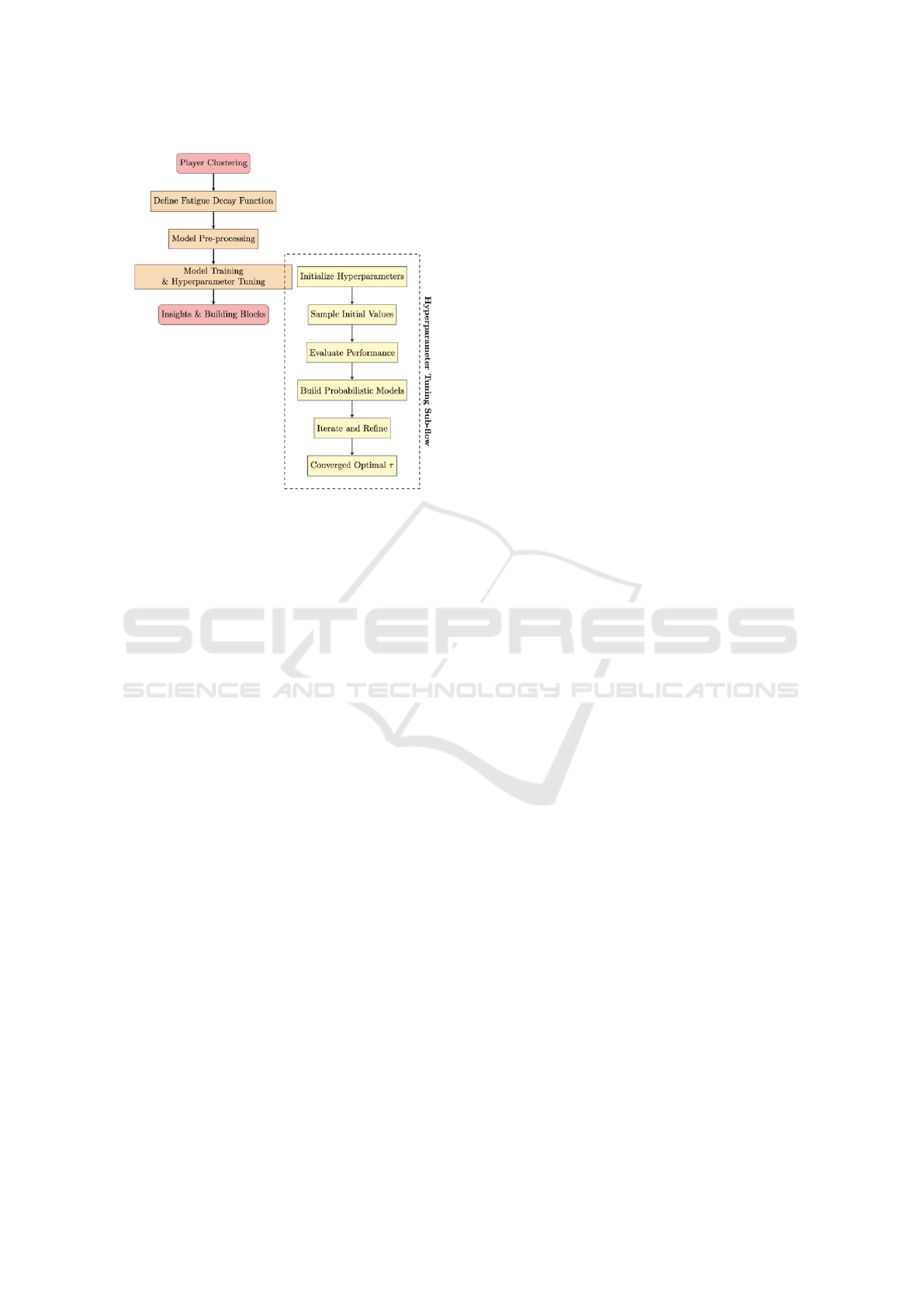
Figure 2: Flowchart for Lineup Optimization Process with

Hyperparemter Tuning Sub-ﬂow, optimizing the tau values

to incorporate within the decay function.

2.7.2 Implementation

The implementation involves iterating over possible

values of τ

and evaluating the performance of the

transformed model. The optimal τ

values are those

that result in the lowest regression error, ensuring that

the model accurately reﬂects the effects of fatigue.

2.8 Player Clustering

To handle high dimensionality and limited data, we

cluster players based on performance characteristics.

These clusters form distinct lineup types, enabling

generalization and robustness in our models. The

method of clustering is open to interpretation in a way

that represents the clusters ideally. For the sake of

this evaluation, the clustering process was performed

based on players’ performances from the previous

year isolated by player. The method in this process of

clustering was K-means , though other methods may

apply as well.

This paper does not focus on the method of clus-

tering, as signiﬁcant work has already been done in

this area. Xu and Martens (Xu and Martens, 2019)

used k-means to group players into roles like ”pri-

mary scorers,” while Terner and Franks (Terner and

Franks, 2016) applied hierarchical clustering to iden-

tify traditional and hybrid positions. Luo and Wu

(Luo and Wu, 2018) further extended this by using

mixed-data clustering for a nuanced view of player ef-

ﬁciency. Building on these established methods, this

paper focuses on the application of these clusters in

lineup optimization.

Clustering players by ”types” and generalizing the

lineups as combinations of ﬁve labels helps to mit-

igate the problem of limited data and high dimen-

sionality. By grouping players with similar perfor-

mance characteristics, we can create more general-

ized lineup types that can be analyzed across multiple

games and teams. This approach allows us to aggre-

gate data from various sources, increasing the robust-

ness and reliability of our models. Additionally, clus-

tering makes the model more adaptable to dynamic

team compositions, ensuring that it remains relevant

even as player rosters change.

3 RESULTS

3.1 Analysis of Optimized τ

Values

The enhanced model, utilizing the optimized τ

values

obtained through the hyperparameter tuning process,

consistently outperforms the baseline model where

no decay function is applied. The optimization of τ

across different data sets has shown to signiﬁcantly

improve predictive accuracy, particularly by captur-

ing the nuances of player performance over time. This

demonstrates that incorporating tailored decay rates

provides a more realistic and effective representation

of fatigue effects within the model.

3.2 Distribution of τ Values Across

Lineups

The analysis across various lineup clusters reveals

that the optimized τ values are distributed unevenly,

with certain lineups exhibiting notably larger τ values

than others. This non-uniform distribution suggests

that different lineups require varying degrees of de-

cay to accurately model performance.

Below , ﬁgure 3 presents the density plot of τ val-

ues, highlighting the variation in decay rates across

different lineups. The plot shows that some lineups

beneﬁt from more aggressive decay (higher τ), lead-

ing to quicker declines in performance, while others

maintain more consistent performance over extended

periods with lower τ values.

3.3 Validation & Improvement Over

Baseline

The improvements gained by applying the optimized

decay functions and τ values are further evaluated by

From Marketing to the Court: Applying MMM and Fatigue Analysis for Optimal Basketball Lineups

129

Figure 3: Density plot of τ values across different lineups,

showing the distribution and variation in optimized decay

rates.

predicting the plus-minus values for each game, based

on the amount of possessions each lineup played,

both with and without the decay function. In this

context, the baseline model represents a regression

without any fatigue function serving as a traditional

linear regression, while the decay functions (kernel-

based) account for player fatigue, dynamically adjust-

ing the contribution of each lineup’s minutes to the

plus-minus metric over time.

In the table below, which presents a comparison of

RMSE values across different decay functions relative

to the baseline model. The table highlights the mean

and median RMSE values, along with their percent-

age improvements. Notably, the majority of the decay

functions outperform the baseline across nearly all tri-

als, with the mean and median values of the exponen-

tial, inverse, and Gaussian decay functions showing

signiﬁcant reductions in error. This strongly indicates

that in most cases, applying the optimized decay func-

tions is preferable, as they consistently lead to better

model performance compared to the baseline.

The Mean RMSE represents the average RMSE

over 20 different folds of the data in a cross validation

comparison.

Table 1: Mean RMSE and % improvement over the baseline

across cross-validation folds using decay functions.

Decay Function Mean RMSE % Improvement

Exponential 4.45 2.79%

Inverse 4.49 2.05%

Gaussian 4.55 0.74%

Baseline 4.58 –

3.4 Optimal Lineups and Fatigue

Management

The results underscore the necessity of managing

player fatigue to optimize overall team performance.

Lineups designed for short bursts of high productivity

can be highly effective in speciﬁc situations but re-

quire careful rotation to prevent rapid declines in per-

formance. Conversely, durable lineups provide steady

performance, making them valuable for maintaining

consistency throughout the game. A team cannot sus-

tain optimal high paced lineups throughout the en-

tire game without ”running out of minutes”. There-

fore one would need to balance between high valued

τ lineups and low valued ones.

4 CONCLUSIONS

This research introduces a comprehensive framework

for optimizing basketball lineups by incorporating the

effects of player fatigue. The integration of decay

functions and sophisticated statistical models offers

coaches data-driven strategies to enhance team perfor-

mance. By balancing productivity and fatigue, teams

can dynamically adjust to in-game conditions and

maintain peak performance throughout the game. The

insights gained have broad implications for the sports

industry, providing a nuanced approach to lineup

management that can give teams a competitive edge.

The analysis reveals signiﬁcant scoring differ-

entials among lineup clusters, demonstrating the

model’s robustness and superiority over baseline ap-

proaches. Optimal lineups exhibit diminishing returns

with prolonged play due to fatigue, underscoring the

need for balanced player utilization.

The insights gained offer coaches data-driven

strategies to enhance team performance. By lever-

aging sophisticated statistical models and clustering

techniques, teams can maintain peak performance and

gain a competitive edge which is well known across

the industry (Stern, 1991). The integration of MMM

principles and fatigue modeling provides a nuanced

approach to lineup management, ensuring optimal

performance throughout games.(Reilly and Williams,

2003)

5 MODEL ASSUMPTIONS AND

LIMITATIONS

While our model demonstrates signiﬁcant improve-

ments over baseline approaches, several key assump-

icSPORTS 2025 - 13th International Conference on Sport Sciences Research and Technology Support

130

tions and limitations warrant discussion, as they both

constrain the current ﬁndings and provide avenues for

future enhancement.

5.1 Decay Function Assumptions

A fundamental assumption of our model is that lineup

performance peaks early and decays monotonically

over time (Fox et al., 2021). This assumption reﬂects

the intuitive understanding that player fatigue accu-

mulates during extended play, leading to diminishing

returns. Future iterations of the model should explore

alternative decay functions, to better capture these nu-

anced performances.

5.2 Variance and Risk Considerations

Our current model focuses on mean performance out-

comes without explicitly accounting for variance in

lineup effectiveness. Two lineups may exhibit identi-

cal mean values but differ signiﬁcantly in their stabil-

ity. This variance component becomes crucial when

considering game situations where certainty of out-

come is crucial, such as close games in the ﬁnal min-

utes. High-variance lineups might be preferred when

trailing signiﬁcantly (requiring high-risk, high-reward

strategies), while low-variance lineups might be opti-

mal when protecting a lead. Incorporating uncertainty

quantiﬁcation into the decay models represents a crit-

ical area of enhancement.

5.3 Clustering Optimization Floor

The player clustering approach, while effective, was

not optimally tuned for this speciﬁc application. We

utilize K-means clustering based on previous season

performance metrics, but this represents a baseline

approach rather than an optimized solution. The ob-

served ∼4% improvement should therefore be viewed

as a performance ﬂoor rather than ceiling. More so-

phisticated clustering methods could yield substan-

tially better player groupings and, consequently, more

accurate lineup optimization. This suggests the true

potential of the methodology may be signiﬁcantly

higher than our current results indicate.

5.4 Strategic Allocation and Game

Planning

Our model provides optimal lineup compositions and

fatigue-adjusted coefﬁcients, but deliberately avoids

prescriptive allocation strategies. The timing and

contextual deployment of speciﬁc lineups remains

within the purview of coaching staff, who must con-

sider factors beyond our model’s scope: opponent-

speciﬁc matchups, foul situations, momentum shifts,

and strategic game ﬂow considerations. This design

choice preserves coaching autonomy while providing

data-driven insights to inform tactical decisions.

5.5 Generalized Data

While validated on Israeli Basketball League data,

the fundamental principles of fatigue accumulation

should remain consistent.

6 DISCUSSION

6.1 Practical Implications Across Time

Horizons

The model’s insights extend across multiple strategic

time horizons, each with distinct implications for bas-

ketball operations:

• Lineup Identiﬁcation: Detecting different lineup

behaviors and identifying which lineups pertain

which characteristics is essential, and a prelimi-

nary step to the full otimization process.

• Short-Term Game Planning: Single game plan-

ning to optimize vs. a given team. Taking into

consideration the current lineup options to maxi-

mize the local horizon.

• Long-Term Roster Construction: The model’s

identiﬁcation of lineup types (high-burst ver-

sus durable) provides strategic insights for roster

building. Teams can evaluate whether their cur-

rent personnel composition aligns with their tac-

tical philosophy and identify speciﬁc player types

needed to complete optimal lineup combinations.

This might inform draft strategies, trade deci-

sions, and free agency priorities by highlighting

whether a team requires more durable role play-

ers or specialized high-impact performers.

6.2 Case Studies

The insights from this model can have a real-world

impact, especially when it comes to making smarter

lineup decisions during games. A couple of notable

examples really bring this to life — the 2016 Golden

State Warriors and the 2014 San Antonio Spurs —

both of which show how our model could inﬂuence

how teams think about lineup choices.

From Marketing to the Court: Applying MMM and Fatigue Analysis for Optimal Basketball Lineups

131

6.2.1 Golden State Warriors (2016 NBA Finals)

In the 2016 NBA Finals, the Warriors stuck with

their “ideal” high-tempo lineup, which on paper gave

them a +15 plus-minus. But the reality the lineup

couldn’t sustain that level of productivity over time.

Fatigue started to take its toll. The model would po-

tentially suggest that swapping Barnes out for Bogut,

while it would’ve dropped the average plus-minus to

+8, could’ve given them a more balanced and sus-

tainable ”marathon” lineup. This trade-off between

short-term peak and long-term productivity is exactly

what our model is designed to capture. So while the

sprint lineup showed higher immediate returns, the

marathon lineup might have been the better call for

the rest of the game.

6.2.2 San Antonio Spurs (2014 NBA Finals)

Now, contrast that with the Spurs in 2014. Even

though Manu Ginobili’s plus-minus (+9) with the

lineup was higher than Danny Green’s (+6), Ginobili

wasn’t a starter. This wasn’t a mistake — it was ac-

tually the right call. Ginobili’s output was great in

short bursts, but as fatigue kicked in, his performance

would’ve dropped. Keeping Green in for more consis-

tent productivity over the full game made more sense.

The model agrees: short-term plus-minus doesn’t al-

ways tell the full story. Sometimes the more durable

lineup, even if less ﬂashy initially, is the one that’s

going to hold up better.

These real-world examples show how the model

could help coaches think beyond just “who’s hot right

now” and focus more on managing fatigue, making

sure the right players are on the court for the right

stretches of the game.

6.3 Future Work

Future work could involve improving the trained

model and decay function. In this paper we can see

the emphasis of the methodology as a breakthrough

for future work. In addition, incorporating oppos-

ing team data to enhance the robustness of the mod-

els. Additionally, exploring more advanced clustering

methods could yield even more precise player group-

ings. Another potential avenue is to apply the mod-

els on a global scale, leveraging data from the entire

league or across multiple leagues, and then tailoring

the insights to optimize individual team strategies.

The improved models developed in this study pro-

vide valuable insights into lineup optimization and

game planning. By converging on more accurate

coefﬁcients, these models facilitate better decision-

making. For instance, while a high-tempo lineup

may show strong initial performance, its effective-

ness can quickly diminish, whereas a lineup designed

for endurance tends to maintain steady performance

throughout the game.

REFERENCES

Fox, J. L., Scanlan, A. T., and Stanton, R. (2021). Peak ex-

ternal intensity decreases across quarters during bas-

ketball games. Montenegrin Journal of Sports Science

and Medicine, 10(1):25–29.

Li, S., Luo, Y., Cao, Y., Li, F., Jin, H., and Mi, J. (2025).

Changes in shooting accuracy among basketball play-

ers under fatigue: a systematic review and meta-

analysis. Frontiers in Physiology, 16:1435810.

Luo, J. and Wu, B. (2018). Player types and efﬁciency in the

nba: A clustering analysis using mixed data. Journal

of Sports Science and Medicine, 17(2):161–169.

Lyons, M., Al-Nakeeb, Y., and Nevill, A. (2006). The

impact of moderate and high intensity total body fa-

tigue on passing accuracy in expert and novice bas-

ketball players. Journal of Sports Science & Medicine,

5(2):215–227.

Macdonald, B. (2012). A regression-based adjusted plus-

minus statistic for nhl players. Journal of Quantitative

Analysis in Sports, 8(3).

NBA (2024). Nba plus-minus: Glossary. Accessed: 2024-

08-24.

Reilly, T. and Williams, A. M. (2003). Science and Soccer.

Routledge.

Rosenbaum, D. T. (2004). Measuring how nba players help

their teams win. In MIT Sloan Sports Analytics Con-

ference.

Sampaio, J. and Janeira, M. (2003). Statistical analyses of

basketball team performance: Understanding teams’

wins and losses according to a different index of ball

possessions. International Journal of Performance

Analysis in Sport, 3(1):40–49.

Stern, H. S. (1991). On the probability of winning a football

game. The American Statistician, 45(3):179–183.

Sullivan, C., Bilsborough, J. C., Cianciosi, M., Hocking, J.,

Cordy, J., and Coutts, A. J. (2014). Match score af-

fects activity proﬁle and skill performance in profes-

sional australian football players. Journal of Science

and Medicine in Sport, 17(3):326–331.

Terner, Z. and Franks, A. (2016). Position and style dif-

ferences among nba players: A clustering approach.

Journal of Quantitative Analysis in Sports, 12(3):145–

160.

Xu, X. and Martens, D. (2019). Clustering nba players: Ex-

amining the inﬂuence of advanced statistics on player

categorization. Journal of Sports Analytics, 5(4):297–

312.

icSPORTS 2025 - 13th International Conference on Sport Sciences Research and Technology Support

132

APPENDIX

The improvements gained by using the optimized

τ values are further illustrated in Table 2, which

presents a comparison of RMSE values across dif-

ferent decay functions relative to the baseline model.

The table highlights the mean and median RMSE val-

ues, along with their percentage improvements. No-

tably, the majority of the decay functions outperform

the baseline across nearly all trials, with the mean and

median values of the exponential, inverse, and Gaus-

sian decay functions showing signiﬁcant reductions

in error. This strongly indicates that in most cases,

applying the optimized decay functions is preferable,

as they consistently lead to better model performance

compared to the baseline.

Table 2: Comparison of RMSE Values for Different Decay

Functions with Mean, Median, and Improvement.

Trial Exp. Inv. Power Gauss. Base

0 4.42 4.49 4.89 4.45 4.53

1 4.50 4.56 4.75 4.55 4.59

2 4.51 4.55 4.77 4.66 4.68

3 4.49 4.53 4.81 4.61 4.62

4 4.13 4.18 4.52 4.33 4.32

5 4.58 4.62 4.90 4.62 4.70

6 4.55 4.60 4.85 4.63 4.66

7 4.31 4.30 4.41 4.40 4.44

8 4.49 4.52 4.77 4.50 4.61

9 4.53 4.56 4.82 4.69 4.71

10 3.75 3.78 4.08 3.82 3.83

11 4.50 4.54 4.60 4.68 4.72

12 4.53 4.56 4.78 4.59 4.63

13 4.57 4.61 4.89 4.69 4.69

14 4.57 4.61 4.90 4.75 4.73

15 4.28 4.33 4.65 4.52 4.46

16 4.51 4.59 4.86 4.61 4.66

17 4.28 4.31 4.61 4.40 4.43

18 4.45 4.49 4.71 4.61 4.62

19 4.39 4.45 4.69 4.48 4.50

Mean 4.45 4.49 4.73 4.55 4.58

Median 4.49 4.52 4.77 4.59 4.62

% Improvement

Mean

2.79% 2.05% -3.21% 0.74% –

% Improvement

Median

2.85% 2.14% -3.25% 0.63% –

From Marketing to the Court: Applying MMM and Fatigue Analysis for Optimal Basketball Lineups

133