Time-Optimal Scheduling of Tasks with Shared and Dynamically
Constrained Energy Systems
Eero Immonen
a
Computational Engineering and Analysis, Turku University of Applied Sciences, Joukahaisenkatu 3-5, Turku, Finland
fi
Keywords:
Task Scheduling, Mixed-Integer Nonlinear Programming, Dynamical Constraints, Energy, Genetic Algorithm.
Abstract:
This article addresses the minimum-time scheduling of sequential tasks requiring energy (or a similar resource)
from shared, dynamically constrained systems. Practical applications of this problem include human opera-
tions with fatigue and rest cycles, among others. The goal is to jointly optimize task execution order and power
allocation to the tasks, balancing execution speed with necessary recovery periods and task transition times.
We present a generic Mixed-Integer Nonlinear Programming (MINLP) formulation of the problem, propose a
heuristic solution method based on a Genetic Algorithm (GA), and demonstrate its use in a numerical example
on efficient execution of a two-exercise workout. The numerical example shows that the proposed heuristic
method rapidly produces a solution within 0.9% of the one obtained via the MINLP solver SCIP.
1 INTRODUCTION
This article addresses the minimum-time scheduling
of sequential tasks that require energy — or other sim-
ilar resource — from shared, dynamically constrained
systems. There are many interesting practical appli-
cations of such scheduling problems. For example,
a team of firefighters, through a collaborative effort
completes physically demanding tasks (e.g. lifting,
digging, carrying) under time constraints. Each task
consumes energy, and the firefighters may need to
rest and recover to be able to undertake the remain-
ing tasks. A structurally similar problem is that of a
high-performance computing system executing a set
of complex computations (e.g. image processing) on
multiple processors, aiming to minimize the total ex-
ecution time in the presence of Ohmic heating. The
computing tasks generate heat that may need to be
dissipated by idling the processors before undertak-
ing subsequent tasks. By Newton’s law of cooling,
such thermal recovery is not immediate.
In both above examples, besides controlling the
task execution order, the operator(s) choose(s) the
power used to engage in the tasks, in order to con-
trol the task execution speed: A higher power yields
a faster task execution time but may later require a
rest-recovery that, on the other hand, causes a delay.
Such task scheduling is thus a tradeoff between local
a
https://orcid.org/0000-0001-5690-287X
and global efficiency. Typically, in practice, there are
also transition times between the tasks, and they are
not necessarily symmetric, i.e. task transition A → B
takes more time than B → A (e.g. climbing stairs up
vs. down).
The purpose of this article is to introduce a generic
mathematical (MINLP) formulation of this problem,
address its heuristic numerical solution by a GA, and
provide a numerical example to illustrate the frame-
work.
2 RELATION TO LITERATURE
Several research articles have addressed time-optimal
task scheduling involving energy consumption, see
e.g. the survey papers (Ghafari et al., 2022) and
(Bambagini et al., 2016) and the references therein.
However, while in these articles the power is a dy-
namical design variable, the objective is to minimize
total energy consumption. Consequently, the energy
system is assumed to be a static resource whose size is
to be minimized for a given set of tasks. As such, this
research typically has targeted an efficient technologi-
cal design, such as low-energy cloud computing envi-
ronment, whereas in the present article we are mainly
interested in efficient human operation.
Efficient human operation is also addressed in the
vast literature on staff rostering (see e.g. (Ngoo et al.,
2022)) and project scheduling (see e.g. (S
´
anchez
Immonen, E.
Time-Optimal Scheduling of Tasks with Shared and Dynamically Constrained Energy Systems.
DOI: 10.5220/0013659100003982
Paper published under CC license (CC BY-NC-ND 4.0)
In Proceedings of the 22nd International Conference on Informatics in Control, Automation and Robotics (ICINCO 2025) - Volume 1, pages 169-175
ISBN: 978-989-758-770-2; ISSN: 2184-2809
Proceedings Copyright © 2025 by SCITEPRESS – Science and Technology Publications, Lda.
169

et al., 2023)). Such research addresses efficient al-
location of finite, static and potentially irreplaceable
resources. These resources are typically equipment
or workforce, but optimal project scheduling with re-
spect to (static) green project indicators (GPIs) i.e.,
energy, noise, and safety, has also been studied (Rah-
man et al., 2022). On the other hand, those articles
that address optimal project scheduling under dynam-
ical resource constraints typically treat them as binary
variables, i.e. disturbances to resource availability;
see e.g. (Xu and Bai, 2024).
In the present article, the objective is to minimize
the execution time of a sequence of tasks constrained
by dynamical energy systems. These energy sys-
tems are described by differential equations that arise
from the seminal theory of human endurance from the
early 1970s. We emphasize, though, that the same
equations can also represent other physical systems
(see Subsection 3.3). This mathematical framework
(Keller, 1973), see also (Pritchard, 1993), for optimal
running is an elegant mix of force balance (for loco-
motion) and power balance (for metabolism) consid-
erations. Indeed, Keller’s model was able to predict
the prevailing world record running times for vari-
ous distances with good accuracy. However, whereas
that model attempts to predict the optimal race times
on flat unidirectional tracks, in the present article we
adapt it to scheduling of different tasks. Moreover,
this article addresses multiple interconnected energy
systems, whereas Keller’s model only has one.
Among those few published articles that, similar
to this paper, address task scheduling under dynami-
cal constraints arising from differential equations, we
mention the work of Zhou et al. (Zhou et al., 2015).
They studied the minimization of energy consumption
of multiprocessor system-on-chip in a schedule dura-
tion, under the constraints of real-time task deadlines
and temperature limit. Their work builds on physics-
based thermal modeling using lumped-parameter sys-
tems. The scheduling problem we consider in this
article is constrained by dynamical energy systems
with recovery, and, instead of minimizing energy con-
sumption, we aim at a minimum-time schedule while
maintaining a nonnegative energy in all systems at all
times.
The problem of time-optimal scheduling of tasks
with shared and dynamically constrained energy sys-
tems is formulated in this article as a MINLP. To
solve it, we propose a heuristic GA-based method.
GAs have been found effective for MINLPs because
they can efficiently explore large, non-convex, and
discontinuous search spaces without requiring gradi-
ent information (Yang, 2020). Their population-based
evolution, through controlled mutation and crossover
operations, allows handling discrete and continuous
variables simultaneously, making them efficient for
the combinatorial and nonlinear structure of MINLPs.
Over the course of the past decades, GAs have been
successfully used in solving task scheduling prob-
lems, including those with energy considerations (see
(Pirozmand et al., 2021) and the references therein).
3 PROBLEM FORMULATION
The optimization problem addressed in this paper in-
volves finding the fastest execution sequence (sched-
ule) for a set of tasks. The time to complete each task
depends on the chosen power, which consumes one or
more dynamical pools of energy.
Although the problem has time-dependent fea-
tures — early decisions influence the future state of
the energy systems — it is formulated in the present
section as a finite-horizon MINLP with nonlinear
state-update constraints. This formulation enables en-
coding discrete task ordering, continuous power allo-
cation, and dynamical resource evolution within a sin-
gle mathematical system (5). The problem displays
aspects of discrete-time optimal control, but due to the
presence of both integer and nonlinear constraints, it
is perhaps best described as an MINLP.
3.1 Definitions
Let i ∈ {1,... ,N} index the tasks t
i
. Let k ∈ {1, ...,n}
index the positions in the task execution sequence,
with n =
∑
N
i=1
M
i
, where M
i
> 0 is the prescribed to-
tal number of tasks of type i in the schedule. Each
task t
i
, i ∈ {1,. ..,N}, requires energy E
i
> 0 to be
completed.
The discrete decision variables (to be optimized)
are the task execution order x
k,i
, with:
x
k,i
=
(
1, if the task at position k is of type i,
0, otherwise,
(1)
such that precisely one task is executed at every posi-
tion, i.e.
∑
N
i=1
x
k,i
= 1, ∀k = 1, .. .,n, and all required
repetitions are carried out, i.e.
∑
n
k=1
x
k,i
= M
i
, ∀i =
1,. ..,N. The continuous decision variables (also to
be optimized) are the task execution powers p
k
∈
[p
min
,P
max
], with 0 < p
min
< P
max
< ∞, k = 1, .. .,n.
At each position k, the chosen power p
k
yields the
execution time d
k
as:
d
k
=
N
∑
i=1
E
i
p
k
x
k,i
(2)
Thus, if the task at schedule position k is of type i
(i.e. x
k,i
= 1), then the task execution time is d
k
=
E
i
p
k
.
ICINCO 2025 - 22nd International Conference on Informatics in Control, Automation and Robotics
170

Transitioning from task t
i
1
to task t
i
2
incurs a delay, as
given by the matrix:
T (i
1
,i
2
) ≥ 0, i
1
,i
2
= 1,. .. ,N. (3)
so that the total execution time of the schedule is
∑
n
k=1
d
k
+
∑
n−1
k=1
T (i
k
,i
k+1
), which is to be minimized.
The choice of power p
k
is constrained by J dy-
namical energy systems, indexed by j ∈ {1,... ,J}.
Each energy system j is updated from the conclusion
of task position k − 1 to the conclusion of the subse-
quent position k > 0 based on the chosen power p
k
:
L
j,k
= min
(
L
j,k−1
+d
k

σ
j
−
∑
i∈I
c
i, j
x
k,i
p
k

, L
max, j
)
,
(4)
where σ
j
is the scalar recovery rate for the energy sys-
tem j, 0 < L
max, j
< ∞ is the maximum energy content
of system j, and 0 ≤ c
i, j
< ∞ is the energy drain coef-
ficient for task i on energy system j ∈ J. Note that the
completion of a task t
i
can require energy from more
than one system j (as in collaborative effort). Initially
L
j,0
> 0, ∀ j ∈ J, and we require all energy systems to
remain non-negative at all times:
L
j,k
≥ 0, ∀ j ∈ J, k = 1, .. .,n.
3.2 Optimization Problem
With the definitions given in Subsection 3.1, the full
optimization problem is:
min
p
k
,x
k,i
n
∑
k=1
d
k
+
n−1
∑
k=1
T (i
k
,i
k+1
) (5a)
s.t. d
k
=
N
∑
i=1
E
i
p
k
x
k,i
, k = 1,...,n, (5b)
L
j,0
> 0, ∀ j ∈ J, (5c)
L
j,k
= min
(
L
j,k−1
+ d
k

σ
j
−
N
∑
i=1
c
i, j
x
k,i
p
k

,
L
max, j
)
, ∀ j ∈ J, k = 1, ...,n,
(5d)
L
j,k
≥ 0, ∀ j ∈ J, k = 1, .. .,n, (5e)
N
∑
i=1
x
k,i
= 1, x
k,i
∈ {0,1}, k = 1,... ,n,
(5f)
n
∑
k=1
x
k,i
= M
i
, ∀i = 1,. ..,N, (5g)
p
k
∈ [p
min
,P
max
], k = 1,...,n. (5h)
3.3 On the Energy System Model
The energy system model in Keller’s theory of com-
petitive running (Keller, 1973) is:
dE
dt
= σ − P, E(0) = E
0
> 0 (6)
where σ > 0 denotes the constant recovery rate and,
by definition, the running power P = f v, i.e. force
times velocity. Equation (4) is a discrete-time anal-
ogy of Equation (6), obtained via a simple Euler in-
tegration (though the integration time is a variable to
be optimized). In Equation (4), also recovery beyond
a finite maximum value is prohibited. Moreover, con-
trary to Keller’s model, in Equation (4), there is not
necessarily a 1 − 1 correspondence between the tasks
and energy systems.
It is important to highlight that the energy Equa-
tion (6) has structurally similar analogs in many other
physical systems. For example, by so-called Coulomb
counting, the State-of-Charge (SoC) of an electric ve-
hicle Lithium-Ion battery can be represented by (Im-
monen and Hurri, 2021):
dSoC
dt
= r −
I
Q
n
, SoC(0) ∈ (0,1] (7)
where r is a regeneration rate, I ≥ 0 is the dis-
charge current and Q
n
is the nominal battery capacity.
Clearly, Equation (7) is Equation (6) for E = SoC,
σ = r and P = I/Q
n
, with I as the design variable.
On the other hand, the Ohmic (Joule) heating of
an electric circuit can be modeled by:
dT
c
dt
= λ(T
amb
− T
c
) + RI
2
, T
c
(0) = T
0
(8)
where R > 0 is resistance, I is electric current, T
amb
−
T
c
is the temperature difference between ambient
(amb) and the circuit (c), and λ > 0 is a coefficient of
heat transfer. Then Equation (8) is just Equation (6)
for E = T
c
, σ = −λT
c
and P = −λT
amb
− RI
2
, with
I as the design variable. The optimization constraint
would be maintaining T
c
(t) ≤ T
max
∀t ≥ 0.
In Equation (7), r is typically dependent on time
(or driving profile or terrain). In Equation (8), the
power term P also has a disturbance (λT
amb
) and the
recovery term σ is not a constant but involves state
feedback from E. Such features may complicate the
numerical solution of Problem (5) under these dynam-
ical constraints. The author expects to address them
in a future article.
Time-Optimal Scheduling of Tasks with Shared and Dynamically Constrained Energy Systems
171

4 HEURISTIC SOLUTION
ALGORITHM
In the Appendix of this article, we describe a GA that,
based on numerical experiments, rapidly yields rea-
sonably good solutions to Problem (5). The method
is described in Algorithm 1, which is based on the two
supplementary methods, Algorithm 2 (mutation) and
Algorithm 3 (crossover). The algorithm implemen-
tations follow the typical structure for genetic algo-
rithms. A slight added complexity arises from ensur-
ing that the population satisfies the constraints (5f)-
(5g) at all times.
5 NUMERICAL EXAMPLE
5.1 Problem Description
Let us consider, as a simple numerical example, the
optimal execution of a physical workout consisting of
two exercises. We seek to determine the minimum-
time execution sequence, and the corresponding pow-
ers, for performing M
1
= 10 squats and M
2
= 10 push-
ups, i.e. i ∈ {1,2 = N} and k ∈ {1,... ,20 = n}.
Each exercise type (i = 1 for squat, i = 2 for push-
up) requires a fixed amount of energy E
i
per repeti-
tion. Based on the change of potential energy, for
a 80 kg person, one squat is assumed to consume
E
1
= 408 J, corresponding to approximately 0.52 m
vertical movement. Similarly, experimental research
reports that standard push-ups use between 69% and
75% of body mass (Ebben and Jensen, 1998). Assum-
ing 71% of 80 kg body mass lifted over 0.45 m, we
obtain the energy consumption E
2
= 250 J for a single
push-up.
Each exercise transition incurs a time penalty, de-
fined by the transition matrix T :
T =

0.5 2.5
5 0.5

(9)
where going up from push-up position to squat posi-
tion T (2,1) takes longer (5 s) than the reverse transi-
tion T (1,2) due to gravity. Repeating either exercise
takes 0.5 s, and it is thus always faster than switching
to the other exercise.
Based on the major muscles activated in the two
workout exercises considered, we assume that the hu-
man body has two energy systems, one for the lower
body ( j = 1) and the other for the upper body ( j = 2).
Both exercises consume energy from both systems but
at different rates, per the drain coefficient matrix c:
c =

1 0.2
0.2 1

(10)
This indicates that a squat (resp. push-up) primarily
consumes energy from the lower (resp. upper) body
energy system, but it also means doing an exercise
makes it more challenging to immediately thereafter
do any exercise. This is consistent with practical ob-
servations from human endurance training.
We assume that the recovery rates are σ
1
= σ
2
=
60 J/s, and that initially the person is fully recovered,
with L
0
= L
max
= [1100,400] J. Finally, we assume
that the maximum power capacity for this individual
is P
max
= 200 W, representing a single muscle group
estimate for an untrained adult (McBride et al., 1999).
5.2 SCIP Global Optimum Solution
To obtain a reference solution to the two-exercise
scheduling problem, the SCIP Optimization Suite 9.0
MINLP solver (Bolusani et al., 2024) was executed
for 2 hours on the CSC Puhti computing environ-
ment. The best feasible schedule found has a to-
tal duration of 78.5 s, with the primal-dual optimal-
ity gap at 0% indicating the global optimum. During
execution, SCIP explored approximately 6.59 mil-
lion nodes, generated 638 feasible solutions, and con-
sumed 10GB of memory.
5.3 Genetic Algorithm Solution
The proposed GA was implemented in Python 3.11
and executed on a laptop workstation with 12th Gen-
eration Intel(R) Core(TM) i7-1265U processor and
32 GB memory. With S
p
= 100 (population size),
G = 3000 (number of generations), µ = 0.2 (muta-
tion rate) and ρ = 0.05 (power change rate), the code
execution completed in less than 2 minutes. The best
execution sequence found by the GA is:
{1,1, 1,1,1
| {z }
Squats
,2, 2,2,2,2,2,2,2
| {z }
Push-ups
,1, 1,1,1,1
| {z }
Squats
, 2, 2
|{z}
Push-ups
}
with a total execution time of 79.2 s.
5.4 Comparison and Discussion
Figure 1 presents a detailed comparison of the opti-
mal solutions obtained by SCIP (Subsection 5.2) and
the proposed GA (Subsection 5.3). Though not iden-
tical, the solutions are very similar: Both favor rep-
etitions of the same exercise once started, to exploit
faster transitions. Moreover, as demonstrated in Fig-
ure 1c and Figure 1d, both schedules first drain all the
energy from the lower body system, then recover that
system to full during 8 push-ups that fully drain the
upper body energy system. The lower body energy
system is then again fully drained in squats, and both
ICINCO 2025 - 22nd International Conference on Informatics in Control, Automation and Robotics
172

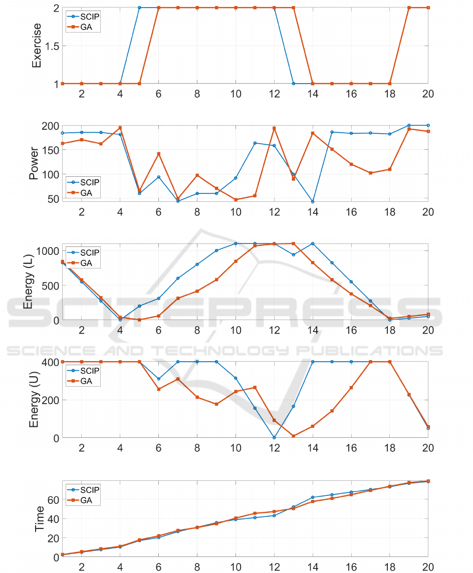
(a) Optimal schedule (1 = Squat, 2 = Push-up)
(b) Power allocation in exercises
(c) Energy in lower body after each exercise
(d) Energy in upper body after each exercise
(e) Cumulative execution time (s)
Figure 1: Comparison of the optimal solutions from SCIP and GA for the numerical example in Section 5. In all plots, the
horizontal axis denotes the task position (k).
Time-Optimal Scheduling of Tasks with Shared and Dynamically Constrained Energy Systems
173

optimal plans finish with the remaining 2 push-ups at
near-maximal power. The cumulative execution time
profiles (Figure 1e) are almost identical, except be-
tween positions 11-16.
The schedule obtained from the proposed GA is
suboptimal. However, the GA solution is obtained
rapidly in comparison to SCIP and the fastest GA
schedule is within 0.9% of the SCIP global mini-
mum. Moreover, the total energy expenditures corre-
sponding to the power assignment schedules of Fig-
ure 1b are: 6579.78 J (SCIP) and 6580.0 J (GA). This
very small difference of 0.003% shows that the SCIP
global optimum power plan is not substantially more
energy efficient either. The proposed GA thus appears
to provide a promising alternative for rapid generation
of high-quality solution candidates for Problem (5).
The workout example addressed herein is perhaps
contrived — it merely aims to illustrate the proposed
GA for solving Problem (5). However, there are well-
known fitness workouts such as Angie in crossfit (Bar-
Bend, 2023) with a similar structure. Solving the cor-
responding optimization problems, as in this section,
would thus also have practical significance in sports
training. Indeed, such optimization results could be
used to design the best strategy for a competition.
They could also be utilized in training to determine
whether improvement in total execution time is due
to increased fitness or just more clever planning of
the workout execution.
6 CONCLUSIONS AND FUTURE
WORK
This article has addressed the minimum-time schedul-
ing of sequential tasks that consume energy from
shared, dynamically constrained systems. We have
presented a general MINLP formulation of the prob-
lem, developed a heuristic solution method based on a
GA, and demonstrated its application, with good per-
formance related to an off-the-shelf solver SCIP, in a
numerical example involving a two-exercise workout.
Perhaps the most interesting future applications of
the mathematical framework presented in this article
are collaborative human scheduling problems, such as
emergency teams. In the future, it also is important
to address minimum-time scheduling problems with
more complex dynamical constraints. As discussed
in Subsection 3.3, one such problem is thermal man-
agement where the dynamical system involves state
feedback. The formalism presented in this article is
easy to adapt to the new domain, but efficient solu-
tion may require further adoption of optimal control
methods.
REFERENCES
Bambagini, M., Marinoni, M., Aydin, H., and Buttazzo, G.
(2016). Energy-aware scheduling for real-time sys-
tems: A survey. ACM Transactions on Embedded
Computing Systems (TECS), 15(1):1–34.
BarBend (2023). How to do the Angie workout in cross-
fit? Available at: https://barbend.com/crossfit-angie-
workout/ (Accessed: 2025-04-03).
Bolusani, S., Besanc¸on, M., Bestuzheva, K., Chmiela,
A., Dion
´
ısio, J., Donkiewicz, T., van Doornmalen,
J., Eifler, L., Ghannam, M., Gleixner, A., et al.
(2024). The scip optimization suite 9.0. arXiv preprint
arXiv:2402.17702.
Ebben, W. P. and Jensen, R. L. (1998). Strength training
for women: Debunking myths that block opportunity.
The Physician and sportsmedicine, 26(5):86–97.
Ghafari, R., Kabutarkhani, F. H., and Mansouri, N. (2022).
Task scheduling algorithms for energy optimization in
cloud environment: a comprehensive review. Cluster
Computing, 25(2):1035–1093.
Immonen, E. and Hurri, J. (2021). Incremental thermo-
electric cfd modeling of a high-energy lithium-
titanate oxide battery cell in different temperatures:
A comparative study. Applied Thermal Engineering,
197:117260.
Keller, J. B. (1973). A theory of competitive running.
Physics today, 26(9):42–47.
McBride, J. M., Triplett-McBride, T., Davie, A., and New-
ton, R. U. (1999). A comparison of strength and power
characteristics between power lifters, olympic lifters,
and sprinters. The Journal of Strength & Conditioning
Research, 13(1):58–66.
Ngoo, C. M., Goh, S. L., Sabar, N. R., Abdullah, S.,
Kendall, G., et al. (2022). A survey of the nurse roster-
ing solution methodologies: The state-of-the-art and
emerging trends. IEEE Access, 10:56504–56524.
Pirozmand, P., Hosseinabadi, A. A. R., Farrokhzad, M.,
Sadeghilalimi, M., Mirkamali, S., and Slowik, A.
(2021). Multi-objective hybrid genetic algorithm for
task scheduling problem in cloud computing. Neural
computing and applications, 33:13075–13088.
Pritchard, W. G. (1993). Mathematical models of running.
Siam review, 35(3):359–379.
Rahman, H. F., Chakrabortty, R. K., Elsawah, S., and Ryan,
M. J. (2022). Energy-efficient project scheduling with
supplier selection in manufacturing projects. Expert
Systems with Applications, 193:116446.
S
´
anchez, M. G., Lalla-Ruiz, E., Gil, A. F., Castro, C., and
Voß, S. (2023). Resource-constrained multi-project
scheduling problem: A survey. European Journal of
Operational Research, 309(3):958–976.
Xu, J. and Bai, S. (2024). A reactive scheduling approach
for the resource-constrained project scheduling prob-
lem with dynamic resource disruption. Kybernetes,
53(6):2007–2028.
Yang, X.-S. (2020). Nature-inspired optimization algo-
rithms. Academic Press.
Zhou, J., Wei, T., Chen, M., Yan, J., Hu, X. S., and Ma,
Y. (2015). Thermal-aware task scheduling for energy
ICINCO 2025 - 22nd International Conference on Informatics in Control, Automation and Robotics
174

minimization in heterogeneous real-time mpsoc sys-
tems. IEEE Transactions on Computer-Aided Design
of Integrated Circuits and Systems, 35(8):1269–1282.
APPENDIX
Algorithm 1: Genetic algorithm for heuristic solution of
Problem (5).
Parameters: S
p
(population size), G
(number of generations), µ > 0 (mutation
rate), ρ > 0 (power change rate).;
Data: i ∈ {1,... ,N}, M
i
, E
i
, σ
j
, c
i, j
,
T (i
1
,i
2
), [p
min
,P
max
].
Result: x
∗
= {x
∗
k,i
} and p
∗
= {p
∗
k
} that
minimize
f (x, p) =
∑
n
k=1
d
k
+
∑
n−1
k=1
T (i
k
,i
k+1
)
subject to Equations (5b)-(5h).
Initialization: Generate initial population
(x, p) ∈ P such that SIZE(P ) = G and:
• x = {x
k,i
} satisfies
∑
N
i=1
x
k,i
= 1, ∀k = 1, .. .,n,
and
∑
n
k=1
x
k,i
= M
i
, ∀i = 1,... ,N.
• p = {p
k
} where p
k
is uniformly randomized
from [p
min
,P
max
].
Initialize f
∗
= ∞.;
for g = 1 to G do
Initialize a new population P
new
=
/
0.;
while SIZE(P
new
) < S
p
do
Parent selection: Randomly select
two pairs (4 candidates) from P and
choose, from each pair, the candidate
with lower f (x, p) as parents, denoted
by (x
1
, p
1
) and (x
2
, p
2
).;
Crossover:
(x
c
, p
c
) ← CROSSOVER

(x
1
, p
1
),(x
2
, p
2
)

mutation:
(x
′
, p
′
) ← MUTATION

(x
c
, p
c
),µ, ρ, p
min
,P
max

Add (x
′
, p
′
) to P
new
.;
end
P ← P
new
.;
Compute f (x, p) for all (x, p) ∈ P .;
if min
(x,p)∈P
f (x, p) < f
∗
then
(x
∗
, p
∗
) ← argmin
(x,p)∈P
f (x, p).;
f
∗
= min
(x,p)∈P
f (x, p).
end
end
return (x
∗
, p
∗
) and f
∗
.
Algorithm 2: Mutation operation for Algorithm 1.
Data: (x, p) ∈ P , µ > 0, ρ > 0, [p
min
,P
max
].
Result: Mutated candidate solution (x
′
, p
′
).
Set x
′
← x and p
′
← p.;
r ← rand([0, 1]).;
if r < µ then
k
1
,k
2
← rand({1,. .. ,n}),k
1
̸= k
2
.;
Swap x
′
k
1
,i
←→ x
′
k
2
,i
, ∀i ∈ 1,... ,N.;
end
for k = 1 to n do
r ← rand([0, 1]).;
if r < µ then
δ ← rand([−ρP
max
,ρP
max
]).;
p
′
k
← max

p
min
,min(p
′
k
+ δ,P
max
)

.;
end
end
return (x
′
, p
′
).
Algorithm 3: Crossover operation for Algorithm 1.
Data: Two parent solutions (x
1
, p
1
) and
(x
2
, p
2
).
Result: Child solution (x
c
, p
c
).
r ← rand({1, .. .,n − 1}).;
For each k = 1,... ,n, set
x
c
k,i
←
(
x
1
k,i
, k ≤ r,
x
2
k,i
, k > r,
∀i = 1, .. .,N.
Let C
i
←
∑
n
k=1
x
c
k,i
∀i = 1,. .. ,N.;
while ∃i ∈ {1, .. .,N} with C
i
> M
i
do
foreach i ∈ {1,... ,N} such that C
i
> M
i
do
D
i
← C
i
− M
i
.;
for d = 1 to D
i
do
k ← rand({ k ∈ {1,...,n} | x
c
k,i
=
1}.;
j ← rand({ j ∈ {1,...,N} | C
j
<
M
j
}.;
x
c
k,i
← 0, x
c
k, j
← 1.;
C
i
← C
i
− 1, C
j
← C
j
+ 1.;
end
end
end
r
2
← rand({1,. .. ,n − 1}).;
For each k = 1,... ,n, set
p
c
k
←
(
p
1
k
, k ≤ r
2
,
p
2
k
, k > r
2
.
return (x
c
, p
c
).
Time-Optimal Scheduling of Tasks with Shared and Dynamically Constrained Energy Systems
175