Leveraging Liquid Time-Constant Neural Networks for ECG

Classiﬁcation: A Focus on Pre-Processing Techniques

Lisa-Maria Beneke

, Michell Boerger

1 a

, Philipp L

ammel

1 b

, Helene Knof

1 c

Andrei Aleksandrov

1 d

and Nikolay Tcholtchev

1,2 e

Fraunhofer Institute for Open Communication Systems (FOKUS), Berlin, Germany

RheinMain University of Applied Sciences, Wiesbaden, Germany

ﬁ

Keywords:

Liquid Time-Constant Neural Networks, LTC, RNN, LSTM, PTB-XL, Time Series Analysis.

Abstract:

Neural networks have become pivotal in timeseries classiﬁcation due to their ability to capture complex tem-

poral relationships. This paper presents an evaluation of Liquid Time-Constant Neural Networks (LTCs), a

novel approach inspired by recurrent neural networks (RNNs) that introduces a unique mechanism to adap-

tively manage temporal dynamics through time-constant parameters. Speciﬁcally, we explore the applicability

and effectiveness of LTC in the context of classifying myocardial infarctions in electrocardiogram data by

benchmarking the performance of LTCs against RNN and LSTM models utilzing the PTB-XL dataset. More-

over, our study focuses on analyzing the impact of various pre-processing methods, including baseline wander

removal, Fourier transformation, Butterworth ﬁltering, and a novel x-scaling method, on the efﬁcacy of these

models. The ﬁndings provide insights into the strengths and limitations of LTCs, enhancing the understanding

of their applicability in multivariate time series classiﬁcation tasks.

1 INTRODUCTION

In the ﬁeld of time series classiﬁcation, neural net-

works have emerged as powerful tools due to their

proﬁciency in capturing complex temporal relation-

ships. The ability to accurately classify tempo-

ral data can lead to signiﬁcant advancements in

predictive analytics and decision-making processes.

Traditional models, such as multilayer perceptrons

(MLPs), convolutional neural networks (CNNs), re-

current neural networks (RNNs), Graph Neural Net-

works (GNNs), and Long Short-Term Memory net-

works (LSTMs) have been studied for timeseries clas-

siﬁcation tasks and have shown promising results.

(Mohammadi Foumani et al., 2024)

More recently, Liquid Time-Constant Neural Net-

works (LTCs) have emerged as a novel approach in-

spired by the principles of RNNs. LTCs introduce a

unique mechanism to adaptively manage temporal dy-

namics through their time-constant parameters. This

https://orcid.org/0000-0002-5741-9043

https://orcid.org/0000-0002-4411-0557

https://orcid.org/0009-0007-1364-6782

https://orcid.org/0000-0002-4717-4206

https://orcid.org/0000-0001-6821-4417

adaptability allows LTCs to model complex temporal

dependencies effectively. (Hasani et al., 2020)

However, the application of LTCs to diverse use

cases remains limited, necessitating a thorough evalu-

ation of their performance against established models

like RNNs and LSTMs. In this paper, we aim to eval-

uate LTCs on a multivariate time series benchmark-

ing dataset from the medical domain. Speciﬁcally, we

want to study their ability to classify myocardial in-

farctions (MI) in electrocardiogram (ECG) data com-

pared to RNN and LSTM models. Additionally, we

want to systematically compare the effectiveness of

various pre-processing methods for this use case. Be-

sides applying common pre-processing methods such

as baseline wander removal, Fourier transformation

and Butterworth ﬁltering, we propose a new x-scaling

method for the task of classifying MI. By doing so, we

seek to provide insights into the strengths and limita-

tions of LTCs, contributing to the broader understand-

ing of their applicability in time series classiﬁcation

tasks. In summary, our key contributions in this paper

are as follows:

• Performance Benchmarking: Comparing the

performance of Liquid Time-Constant Neural

Networks against RNNs and LSTMs for myocar-

234

Beneke, L.-M., Boerger, M., Lämmel, P., Knof, H., Aleksandrov, A., Tcholtchev and N.

Leveraging Liquid Time-Constant Neural Networks for ECG Classiﬁcation: A Focus on Pre-Processing Techniques.

DOI: 10.5220/0013648000003967

In Proceedings of the 14th International Conference on Data Science, Technology and Applications (DATA 2025), pages 234-245

ISBN: 978-989-758-758-0; ISSN: 2184-285X

dial infarction classiﬁcation using the PTB-XL

dataset.

• Analysis of Pre-processing Techniques: Ex-

amination of the effects of various signal pre-

processing methods, including baseline wander

removal, Fourier transformation, Butterworth ﬁl-

tering, and a novel x-scaling technique on models’

performance on classifying temporal relations.

• Insights on LTC Applicability: Exploring the

applicability of LTCs in a real-world use case

while identiﬁng the strengths and limitations of

LTCs in multivariate time series classiﬁcation,

contributing valuable insights for future research

and practical applications in medical diagnostics.

The reminder of this paper is structured as follows:

Section 2 provides a background on LTCs and related

models, followed by a detailed description of the ex-

perimental setup in Section 3. Section 4 analyzes the

impact of various pre-processing methods on model

performance, while Section 5 discusses hyperparam-

eter optimization and presents the ﬁnal MI detection

models. Finally, Section 6 concludes with insights

from the study and future work directions.

2 BACKGROUND AND STATE OF

THE ART

This section provides an overview of Liquid Time-

Constant Neural Networks (LTCs) and their rela-

tionship with Neural Ordinary Differential Equations

(Neural ODEs) and Continuous-Time Recurrent Neu-

ral Networks (CT-RNNs). We will outline the funda-

mental principles of these models and their distinc-

tive characteristics. In addition, we will present the

latest related work on the utilisation of ML-based ap-

proaches for MI detection.

2.1 Neural Ordinary Differential

Equations

The use of ordinary differential equations (ODEs) in

modeling dynamic systems is motivated by their abil-

ity to capture continuous-time behavior and complex

temporal relationships. Neural ODEs extend this con-

cept by incorporating neural networks into the frame-

work, allowing for ﬂexible and expressive modeling

of system dynamics. Given a neural network function

f that is parameterized by θ (i.e. weights and biases),

the state x(t) of the modelled system at time t is de-

ﬁned by the Ordinary Differential Equation

Figure 1: Illustration of a cell i ∈ [1, ..., m] of an LTC with

weights w

i j

, w

contained in Θ, and connected neu-

rons l, j ∈ [1, ..., m], i ̸= l and i ̸= j

dx(t)

= f (x(t), t, θ)

where I(t) denotes external inputs to the system

(Chen et al., 2018).

2.2 Continuous-Time Recurrent Neural

Networks

CT-RNNs also model temporal dynamics using dif-

ferential equations. The state update is given by:

dx(t)

= −

x(t)

+ f (x(t), t, θ)

The key difference between CT-RNNs and Neural

ODEs lies in the inclusion of the term −

x(t)

, which

stabilizes the system and helps it reach an equilibrium

state with a speciﬁc time constant τ. (Funahashi and

Nakamura, 1993)

2.3 Liquid Time-Constant Neural

Networks

Hasani et al. (Hasani et al., 2020) propose yet another

formula in which the neural network not only deter-

mines the derivative of the state x but also serves as

an input-dependent varying time-constant:

dx(t)

= −

x(t)

+ f (x(t), t, θ) (A − x(t))

with θ and A being parameters. As described above,

CT-RNNs calculate an ODE with a time constant

∈ R, i ∈ N for every i-th unit in the neural net-

work. Contrary to that, LTCs are utilising varying

(i.e. liquid) time-constants coupled to their hidden

state. This improves ﬂexibility and adaption of the

network, especially on time-series prediction tasks

Leveraging Liquid Time-Constant Neural Networks for ECG Classiﬁcation: A Focus on Pre-Processing Techniques

235

Table 1: PTB-XL based related work results.

Literature Year Classiﬁers Accuracy AUC

Smigiel et al. (

Smigiel et al., 2021) 2021 CNN 72.0% -

SincNet 73.0% -

Smigiel et al. (

Smigiel et al., 2021) 2021 Neural Networks 76.2% -

Pa’lczynski et al. (Pałczy

nski et al., 2022) 2022 Neural Networks 80.2% -

Prabhakararao et al. (Prabhakararao and Dandapat, 2022) 2022 DMSCE 84.5% -

Anand et al. (Anand et al., 2022) 2022 CNN 93.4% -

Knof et al. (Knof et al., 2024a) 2024 CNN 96.21% 98.91%

Strodthoff et al. (Strodthoff et al., 2021) 2021 LSTM - 90.7%

xresnet1d - 92.5%

inception1d - 92.5%

(Hasani et al., 2020). The general structure of a single

unit i ∈ [1, ..., m] is outlined in Figure 1.

Compared to existing algorithms, LTCs promise

to better capture the causality in data patterns over

time, while being much more robust and expressive.

They demonstrate stable and bounded behavior, offer

enhanced expressivity among neural ODEs (i.e., time-

constant neural networks), and result in better perfor-

mance on time series prediction tasks (Hasani et al.,

2020).

2.4 Related Work

In the following, we will discuss related ML-based

approaches for the detection of myocardial infarctions

based on multivariate ECG timeseries data, which are

summarized in Table 1.

The most dominant method of solving MI de-

tection of 12-lead ECG data utilises Convolutional

Neural Networks to classify between MI and non-

MI classes. (Acharya et al., 2017) (Gharaibeh and

Quwaider, 2022) (Atiea and Adel, 2022) Further-

more Segura-Saldana et al. (Segura-Salda

na et al.,

2022), Xiong et. al (Xiong et al., 2022), Joloudari

et al. (Joloudari et al., 2022) and Lynn et al. (Lynn

et al., 2019) showed that Gated Recurring Units and

LSTMs are used for MI and non-MI classiﬁcation

as well. Many approaches like (Singh et al., 2018)

and (Muhuri et al., 2020) utilise a multi-layer LSTM

model for accurately classifying time-series into mul-

tiple classes. Since LTCs are based on recurrent net-

works, like LSTM, these results give good insights

into the expected performance.

Hammad et al. (Hammad et al., 2022) compared

multiple models for MI detection, which a relevant

amount of is based on the PTB-XL dataset, described

in Section 3.1. As it can be seen in Table 1, Anand

et al. (Anand et al., 2022) achieved results of up to

93.4% classiﬁcation accuracy.

Like others, Rai et al. (Rai and Chatterjee, 2022)

additionally utilised a combination of multiple mod-

els, for example Convolutional Neural Networks and

LSTM to further improve the results. They were

achieving detection accuracies on a combination of

multiple datasets of up to 99.89%.

Another study by Knof et al. (Knof et al., 2024a)

developed a CNN model to detect indications of my-

ocardial infarction based on ECG data. Further, they

aimed to explain and evaluate the model’s decision-

making process using explainable AI methods (Knof

et al., 2024b). They also utilised the PTB-XL dataset

and reported an MI detection performance of 96.21%

accuracy and AUC of 98.91% for their CNN model.

Strodthoff et al. (Strodthoff et al., 2021) compared

the performance of various state of the art machine

learning algorithms for the MI detection use case

based on ECG measurements as a benchmark, specif-

ically optimised for the PTB-XL data set (Wagner

et al., 2020). Unfortunately they provide their results

in AUC measurement only, which makes it hard to di-

rectly compare them to the other results in Table 1.

The comparison from Strodthoff et al. (Strodthoff

et al., 2021) focuses on different approaches of mul-

tilabel and binary classiﬁcation, as well as regression

tasks. Comparing the results with our work, mostly

the results of the multilabel classiﬁcation of the diag-

nostic ECG statements are relevant, since they come

close to the use case of a binary classiﬁcation between

MI and non-MI diagnostic ECG statements.

Comparably to this paper, Strodthoff et al.

(Strodthoff et al., 2021) utilised both the raw ECG

signal and a feature-based approach for the classi-

ﬁcation. Interestingly they showed that many re-

sults of the image classiﬁcation domain can be trans-

ferred into the time-series classiﬁcation domain. They

showed that the newly proposed xresnet1d101 model

performed best in all experiments - with a 93.7% AUC

value on the classiﬁcation of ECG diagnostics.

In comparison to existing work, this paper stands

out as the ﬁrst to utilize LTCs for the detection of

myocardial infarctions, demonstrating their applica-

bility in a critical medical context. Additionally, it

presents a comprehensive evaluation of various pre-

processing methods tailored for noisy ECG timeseries

DATA 2025 - 14th International Conference on Data Science, Technology and Applications

236

PTB-XL

Windowing

Encoding

Splitting

Data Preparation

Applying Signal

Pre-processing

Te ch ni qu es

Evaluate Pre-

Processing

Techniques

Final Data

Tran s f o r m a t io n :

Select & Apply

Pre-Processing

Technique( s )

on prepared

Data

Model & Hyper-

parameter

Optimization

Evaluate

Model

Build

MI Detection

Models

Balancing

Butterworth

Filtering

Baseline

Wander

Removal

Fourier Trans-

formation

X-Axis Scaling

Figure 2: Methodology followed to analyse the effect of

pre-processing techniques, and train and build MI detection

models utilzing neural ODEs.

data, highlighting the novel x-scaling approach de-

veloped speciﬁcally for this task (see Section 3.3.4).

This thorough analysis not only contributes to the

current understanding of LTCs, but also offers valu-

able insights into the optimization of pre-processing

techniques for improved classiﬁcation performance in

ECG signal analysis.

3 EXPERIMENTAL SETUP

To demonstrate and validate the performance of LTCs

in real-world applications, we apply them to a medical

use case, comparing their effectiveness with RNNs

and LSTMs. Speciﬁcally, we focus on classifying

myocardial infarction (MI) using 12-lead electrocar-

diogram (ECG) data and investigate the impact of var-

ious pre-processing methods. Throughout the exper-

iments, we adhered to the methodology depicted in

Figure 2, which we will outline in the following sec-

tions.

3.1 Description of Dataset

We utilize the PTB-XL benchmarking dataset (Wag-

ner et al., 2020), which contains 21.799 ECG records

of 10 seconds length, organized into stratiﬁed train-

ing, validation, and test sets. Each ECG record is

labelled with one of ﬁve superclasses: NORM, CD,

HYP, STTC, and MI.

3.2 Data Preparation

In the following, we outline the data preparation

phase, which includes essential steps such as data en-

coding, windowing, class balancing, and splitting, all

consistently applied in our experiments.

Figure 3: Data windowing.

3.2.1 Encoding

In our use case, we focus on the detection of MI

within ECG records. Therefore, we relabel all ECG

records belonging to a different class than MI with

non-MI. Additionally, we apply one-hot encoding,

such that the models output 1 when deciding for MI

and 0 otherwise.

3.2.2 Windowing

Neural networks typically require ﬁxed-length inputs

for class prediction. To facilitate continuous classi-

ﬁcation of time series data, we standardize the win-

dow length across our dataset by segmenting the 10-

second ECG recordings from the training set into

multiple smaller windows of ﬁxed length, with a de-

fault length of 5 seconds. These windows may over-

lap to create additional training data and are evenly

distributed across the entire recording, with the ﬁrst

window aligned to the start and the last window

aligned to the end of the data stream. Figure 3 demon-

strates how a single input data stream is divided into

four distinct windows.

3.2.3 Class Balancing

Models can be biased towards the majority class when

the training set is imbalanced (Krawczyk, 2016). In

our dataset, the number of MI-labeled recordings is

with 4.192 signiﬁcantly lower than that of non-MI

recordings which is 17.607. This class imbalance is

particularly critical in medical contexts such as MI

prediction, where the minority class (i.e., MI) holds

substantial clinical signiﬁcance. To address this im-

balance, we employ a data-level method that gener-

ates overlapping windows from the MI recordings, al-

lowing for the augmentation of the training set and

thereby increasing the representation of the minority

class (Krawczyk, 2016). Figure 4 illustrates how the

number of windows is increased by a factor of 1.5.

Figure 4: Balancing with overlapping windows.

Leveraging Liquid Time-Constant Neural Networks for ECG Classiﬁcation: A Focus on Pre-Processing Techniques

237

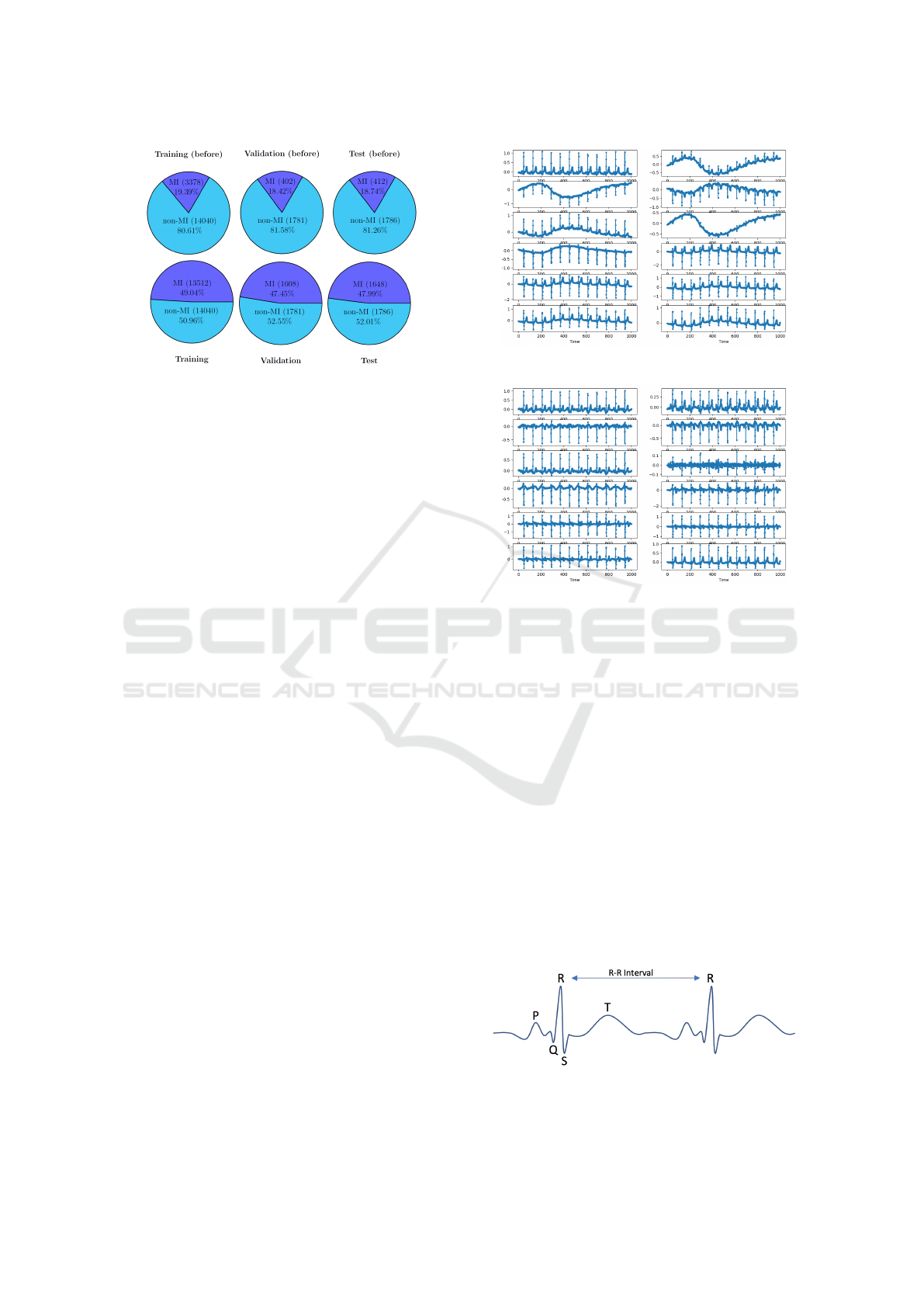
Figure 5: Distribution per class before and after balancing.

Applying this sliding-window approach to the whole

dataset, we obtain a training set of 27.552 recordings

(13.512 MI and 14.040 non-MI), a validation set of

3.389 recordings (1.608 MI and 1.781 non-MI), and

a test set of 3.434 recordings (1.648 MI and 1.786

non-MI). The distribution before and after balancing

is depicted in Figure 5.

3.3 Data Pre-Processing Techniques

Subsequently, we present pre-processing methods ap-

plied to the encoded and balanced dataset, including

baseline wander removal, x-scaling, Butterworth ﬁl-

tering, and Fourier transformation. We will evaluate

the impact of these methods on model training by ap-

plying and analyse all possible combinations of the

selected pre-processing techniques (see Section 4).

3.3.1 Baseline Wander Removal

ECG measurements can be affected by various fac-

tors of external noise on the electrode, such as ﬁn-

ger movement or other external inﬂuences (Sargolzaei

et al., 2009)(Degerli et al., 2021). A common source

of noise in these measurements is known as baseline

wander. This phenomenon occurs when the center of

the ECG signal deviates from a zero baseline and in-

stead follows an underlying curve. For example, the

top right lead in Figure 6 exhibits a sinusoidal pat-

tern over the ﬁrst 7 seconds of data. Sargolzaei et al.

(Sargolzaei et al., 2009) proposed an algorithm to en-

hance the data quality of ECG measurements for ma-

chine learning applications. This algorithm iteratively

computes the wavelet transformation of the original

ECG signal, after which it reconstructs the baseline

of the ECG signal using an inverse wavelet transfor-

mation. Figure 6 displays the measurements of the

12 leads prior to applying the algorithm proposed by

Sargolzaei et al. (Sargolzaei et al., 2009), revealing a

noticeable wandering baseline across nearly all leads.

Figure 6: 12 ECG leads before BWR.

Figure 7: 12 ECG leads after BWR.

In contrast, Figure 7 illustrates the clarity of the signal

following the application of the algorithm.

3.3.2 R-Peak Detection

Each heartbeat exhibits several key indicator points,

as shown in Figure 8. The R-peak is typically the

most prominent amplitude in the ECG measurement,

reﬂecting the heart’s contraction as it pumps blood

throughout the body (S and Morris, 2002).

The Pan-Tompkins QRS-Detection algorithm

(Pan and Tompkins, 1985) identiﬁes R-peaks in ECG

recordings. This algorithm incorporates a series of

ﬁltering and processing steps designed for effective

noise reduction. Speciﬁcally, it employs a low-pass

and high-pass ﬁltering technique, which is compa-

rable to the Butterworth ﬁlter described in Section

3.3.6. However, unlike the Butterworth ﬁlter, the Pan-

Tompkins noise cancellation ﬁlter is typically imple-

Figure 8: Sketch of an idealised ECG Lead-1 measurement.

Own representation based on (Singh et al., 2018).

DATA 2025 - 14th International Conference on Data Science, Technology and Applications

238

mented in a recursive manner for any arbitrary but

ﬁxed time-step t ∈ R.

Let f denote the ECG signal. The low-pass ﬁlter

low

: R → R and the high-pass ﬁlter f

high

: R → R are

deﬁned as follows:

low

(x) := 2 f

low

(x −t) − f

low

(x − 2t)

+ f (x) − 2 f (x − 6t) + f (x − 12t)

high

(x) := 32 f (x − 16t) − f

high

(x −t)

− f (x) + f (x − 32t)

For negative time values, the functions for the

ECG signal and both ﬁlters equal zero. This approach

ensures that there is no output for time points that do

not exist in the signal.

These ﬁlters then calculate the noise-ﬁltered sig-

nal s : R → R:

˜s(x) := f

high

( f

low

( f (x)))

s(x) :=

˜s(x)

max(| ˜s(x)|)

In the following step, the algorithm computes the

derivative of this ﬁltered signal, and the result is

squared. This processed data stream is then aver-

aged over a moving window of 150 ms, facilitating

the identiﬁcation of approximate R-peaks.

As an optimization to this algorithm, a ”climb-the-

hill” approach is applied after detecting the R-peaks

with the Pan-Tompkins algorithm. This technique

checks if an identiﬁed R-peak can adjust left or right

to increase its value. If this adjustment is possible,

the R-peak repositions until any movement in either

direction results in a decreased value of the function.

The ”climb-the-hill” optimized Pan-Tompkins

QRS-Detection algorithm demonstrates promising re-

sults, although it occasionally misidentiﬁes T-waves

as R-peaks. For an example of accurate identiﬁcation,

see Figure 9. For an instance where a T-wave is incor-

rectly identiﬁed to be an R-peak, refer to Figure 10.

Each ﬁgure illustrates data from the ﬁrst four steps of

the Pan-Tompkins algorithm outlined earlier (band-

pass ﬁlter, derivative, squaring, moving average) and

marks the identiﬁed approximate R-peaks with a pink

cross on the original input data in the bottom plot.

3.3.3 Y-Axis Scaling

To normalize the data, the Scikit Learn Standard-

Scaler is used. The scaler takes all ECG recordings

from the training dataset, calculates the average value

and variance, and uses this to transform all ECGs of

the whole dataset. This generates ECG recordings

which are centered around 0 and with variance 1.

Figure 9: Correctly identiﬁed R-peaks.

Figure 10: Wrongly identiﬁed R-peaks.

3.3.4 X-Axis Scaling

We propose an x-scaling technique optimized for this

speciﬁc use case. The underlying concept of this scal-

ing addresses the issue that medical health data does

not remain within a static frequency domain; instead,

the frequency varies over time, as exempliﬁed by the

non-constant nature of heart rate. Through x-scaling,

or time-scaling, the data is transformed into a format

that accounts for these temporal variations. Given that

this approach is not a conventional algorithm, we pro-

vide a detailed explanation of the concept and its im-

plementation, as outlined in Algorithm 1.

The x-scaler is speciﬁcally designed for ECG

recordings, as it relies on detecting and aligning heart-

beats within the observed data. To transform the

data, the algorithm iterates over all data points in

the time-series window to identify the heartbeats us-

ing the Pan-Tompkins QRS Detection algorithm (Pan

and Tompkins, 1985). Although the Pan-Tompkins

algorithm operates independently for each lead, all

12 leads in this use case correspond to measurements

from a single heart. Therefore, additional steps are

taken to determine the most likely heartbeat time

points in each recording from all 12 leads. First, the

Figure 11: X-scaling of a 4-second window.

Leveraging Liquid Time-Constant Neural Networks for ECG Classiﬁcation: A Focus on Pre-Processing Techniques

239

Algorithm 1: Scaling Beats (x-axis scaling).

1: for i = 0 to len(beats) − 2 do

2: di f f erence ← beats[i + 1] − beats[i]

3: rate ←

sampling rate

di f f erence

4: for j = 0 to di f f erence − 1 do

5: k ← i ∗ sampling rate + int(round( j ∗ rate))

6: n ← i ∗ sampling rate + int(round(( j + 1) ∗

rate))

7: m ← beats[i] + j

8: if n ≥ len(records) then

9: continue

10: end if

11: # Standard case

12: if n − k = 1 then

13: scaled[k] ← records[m]

14: scaled[n] ← records[m + 1]

15: # Squashed to single index:

16: # take average value

17: else if k = n then

18: scaled[k] ←

records[m]+records[m+1]

19: # Stretched to three indexes:

20: # take average value as

21: # additional middle point index

22: else if n − k = 2 then

23: scaled[k] ← records[m]

24: scaled[k + 1] ←

records[m]+records[m+1]

25: scaled[n] ← records[m + 1]

26: end if

27: end for

28: end for

results from the Pan-Tompkins QRS detection are col-

lected, and the number of detected heartbeats per lead

is counted across the entire time window as can be

seen in Figure 12a. The dominant count of heartbeats

per lead is identiﬁed, and any leads exhibiting a differ-

ent number of beats are excluded from further analy-

sis (see Figure 12b). For the remaining selected leads,

the time points of the detected heartbeats are averaged

to establish a consensus on the overall heartbeat (see

Figure 12c). The ﬁnal detected heartbeats are visual-

ized in Figure 12d.

Following this detection, the algorithm stretches

or compresses each heartbeat along the x-axis to en-

sure exactly one heartbeat is represented per ”sec-

ond”. This adjustment guarantees a constant recur-

rence rate in the data. The process for scaling a 4-

second window of irregular data to a regular pattern

is visualized in Figure 11.

As illustrated in Algorithm 1, the scaling process

begins by calculating the total number of time steps

between beat i and i + 1. The sampling rate is then

divided by this number to determine a scaling rate,

which indicates how far the points need to be com-

pressed or stretched in time. Since the data points

are stored in memory as an array, we cannot simply

move the x-axis points around; instead, we approxi-

mate their positions by rounding to the next integer

value. This approximation can introduce a timing er-

ror of up to half the sampling rate per second (e.g.,

up to 5 ms for a 100 Hz sampling rate). However,

with error rates of 0.5% or 0.1%, we consider this

error to be sufﬁciently small for the given use case,

outweighed by the beneﬁts of the transformation.

After calculating the scaling rate, we iterate over

each point for each heartbeat interval. Each point is

scaled by the scaling rate and mapped onto the next

integer value. If two points project onto the same in-

dex, the average value between those points is stored

at that index. If two points project to non-adjacent in-

dexes, intermediate points are ﬁlled with a linear in-

terpolation between the two scaled points.

This procedure can be applied to a continuous

stream of data. However, a limitation is that the win-

dow lengths of each dataset might differ. To address

this, all datasets are truncated to the same length dur-

ing preprocessing, speciﬁcally to the length of the

shortest processed dataset. We expect this transforma-

tion to yield improved results, as the machine learn-

ing algorithm will focus on classifying anomalies in

the heartbeat without needing to adapt to linear trans-

formations over time. It is important to note that this

approach may result in the loss of information based

on the frequency of the heartbeat.

(a) ECG with detected R-

peaks per lead

(b) 5 selected leads of ECG

with R-peak detection

with heartbeat detection

(d) ECG with heartbeat de-

tection per lead

Figure 12: ECG lead analysis.

DATA 2025 - 14th International Conference on Data Science, Technology and Applications

240

3.3.5 Fourier Transformation

A Fourier Transformation analyzes a function by ex-

tracting the amplitude and frequency of its underly-

ing structure. It generates a new function that de-

picts spikes of amplitude at corresponding frequency

points. However, this transformation does not retain

temporal shifts; thus, two functions that are identi-

cal except for their position along the x-axis yield the

same Fourier Transformation. To address the limita-

tion of identifying trends over time, the Short-Time

Fourier Transform (STFT) is employed, which di-

vides the raw input data into short time intervals as

explained in (Dey et al., 2021). A Fourier Transfor-

mation is then applied to each interval, resulting in

a two-dimensional representation that illustrates the

amplitude of various frequencies across time.

3.3.6 Butterworth Filter

The Butterworth ﬁlter is utilized to selectively ﬁlter

out frequencies outside a speciﬁed range. In this im-

plementation, a lower threshold of 20Hz and an up-

per threshold of 200Hz are chosen. These thresh-

olds are appropriate for ECG measurements, which

correspond to the rhythm of human heartbeats, typ-

ically occurring within this frequency range (Naseri

and Homaeinezhad, 2012).

3.4 Description of Models

To evaluate the effectiveness of the four pre-

processing approaches presented, we compare the

performance of an LTC against RNN and LSTM mod-

els. Each model’s architecture is minimalistic, with

a limited number of connected layers, to ensure a

clear performance comparison following various pre-

processing steps. All models accept batched time-

series input structured as a three-dimensional tensor

with the shape (batch size, number of features, num-

ber of timesteps). We set the batch size to 32, the

number of features to 12 (corresponding to the 12

leads in each ECG recording), and the number of

timesteps to 500. The input tensor is processed by a

TensorFlow base layer, where the cell type is deﬁned

as either RNN, LSTM, or LTC. The output of this base

layer is then passed to a dense layer, producing a sin-

gle output that indicates the prediction score for My-

ocardial Infarction. For training the models, we use

the Adam optimizer with a learning rate of 0.005 for

LTCs and 0.001 for LSTMs and RNNs, following the

guidelines provided by the authors in (Hasani et al.,

2020). For each conﬁguration of pre-processing steps,

we train all three models for 100 epochs and compare

their accuracy, precision and recall using the valida-

tion set of the PTB-XL dataset.

Afterwards, we will select the best-performing

pre-processing techniques based on the obtained re-

sults, and train and optimise ﬁnal models for the de-

tection of MIs, which will be then evaluated on the

train set (compare Figure 2). This approach and the

associated models are discussed in Section 5.

4 ANALYZING THE EFFECT OF

PRE-PROCESSING

TECHNIQUES

Table 2 displays the performance metrics accuracy,

precision, and recall of the trained LTC, LSTM, and

RNN models for the four investigated pre-processing

approaches on the validation set. The pre-processing

steps are indicated by crosses (disabled) and ticks (en-

abled). We evaluate all possible combinations of the

four pre-processing steps x-scaling (XS), Butterworth

ﬁltering (BF), Fourier transformation (BF) and base-

line wander removal (BWR). The performance met-

rics are based on the validation set after training the

models on the training set for 100 epochs.

The LSTM has an average accuracy of 0.7608,

outperforming the LTC and RNN, which have average

accuracies of 0.7319 and 0.7064, respectively. Fur-

thermore, the LSTM achieves a higher average pre-

cision of 0.7691, compared to the LTC’s 0.7034 and

the RNN’s 0.6624. In terms of average recall, the LTC

leads with 0.7616, followed by the LSTM at 0.6959

and the RNN at 0.4465. This indicates that the RNN

is not that effective as the LSTM and the LTC for

the task of detecting myocardial infarctions in 12-lead

ECG recordings. We observe the following for the

impact of the four pre-processing steps.

1) X-Scaling signiﬁcantly enhances performance.

As shown in Table 2, conﬁgurations with enabled x-

scaling outperformed those with it disabled, with only

one exception. For LSTM, the x-scaling enabled con-

ﬁgurations averaged 5.28% higher in accuracy. The

RNN conﬁgurations demonstrated an even greater in-

crease of 11.47%. In contrast, the LTC conﬁgurations

showed a modest improvement of 1.98%.

2) There are no signiﬁcant improvements ob-

served from enabling BWR. Indeed, it often results

in a decrease in the model’s accuracy as can be ob-

served from Table 2. When all pre-eprocessing steps

are ﬁxed except for BWR, the LTC model shows a de-

cline in accuracy in ﬁve cases, while only two cases

exhibit an increase. Similarly, the RNN model experi-

ences a decrease in ﬁve cases and an increase in three

Leveraging Liquid Time-Constant Neural Networks for ECG Classiﬁcation: A Focus on Pre-Processing Techniques

241

Table 2: Validation set accuracy, precision and recall for all

conﬁgurations of the investigated pre-processing methods

XS BF FT BWR Model Accuracy Precision Recall

LTC 0.790 0.819 0.649

✗ ✗ ✗ ✗ LSTM 0.732 0.730 0.714

RNN 0.626 0.539 0.420

LTC 0.756 0.762 0.725

✗ ✗ ✗ ✓ LSTM 0.780 0.764 0.797

RNN 0.650 0.630 0.623

LTC 0.743 0.715 0.791

✗ ✗ ✓ ✗ LSTM 0.739 0.745 0.718

RNN 0.680 0.589 0.675

LTC 0.780 0.751 0.817

✗ ✗ ✓ ✓ LSTM 0.750 0.774 0.660

RNN 0.672 0.656 0.612

LTC 0.739 0.715 0.785

✗ ✓ ✗ ✗ LSTM 0.724 0.737 0.630

RNN 0.649 0.587 0.377

LTC 0.715 0.671 0.784

✗ ✓ ✗ ✓ LSTM

- - -

RNN 0.645 0.524 0.381

LTC 0.645 0.557 0.852

✗ ✓ ✓ ✗ LSTM 0.708 0.708 0.560

RNN 0.607 0.542 0.546

LTC 0.629 0.575 0.696

✗ ✓ ✓ ✓ LSTM 0.700 0.681 0.689

RNN 0.664 0.608 0.271

LTC 0.761 0.760 0.739

✓ ✗ ✗ ✗ LSTM 0.801 0.837 0.699

RNN 0.788 0.715 0.441

LTC 0.792 0.800 0.778

✓ ✗ ✗ ✓ LSTM 0.814 0.838 0.711

RNN 0.792 0.817 0.306

LTC 0.750 0.709 0.806

✓ ✗ ✓ ✗ LSTM 0.801 0.821 0.709

RNN 0.731 0.643 0.620

LTC

- - -

✓ ✗ ✓ ✓ LSTM 0.801 0.825 0.730

RNN 0.771 0.768 0.348

LTC 0.773 0.693 0.863

✓ ✓ ✗ ✗ LSTM 0.769 0.779 0.724

RNN 0.777 0.750 0.545

LTC 0.636 0.576 0.802

✓ ✓ ✗ ✓ LSTM 0.775 0.785 0.693

RNN 0.757 0.770 0.302

LTC 0.742 0.700 0.793

✓ ✓ ✓ ✗ LSTM 0.764 0.751 0.711

RNN 0.767 0.768 0.353

LTC 0.730 0.750 0.545

✓ ✓ ✓ ✓ LSTM 0.754 0.761 0.694

RNN 0.728 0.693 0.326

cases

. In contrast, the LSTM model demonstrates

a greater number of instances where enabling BWR

enhances the model’s accuracy.

3) The use of the Butterworth Filter in the pre-

processing phase generally results in decreased accu-

racy. Speciﬁcally, there are no conﬁgurations where

Note that there is one case more for the RNN model

than for the LTC model due to data loss.

it improves the accuracy of the LSTM model. For the

LTC and RNN models, it only enhances performance

in one and two cases, respectively.

4) Applying the Fourier transformation also leads

to a decrease in the models’ accuracies in most cases.

This holds true for the LTC, LSTM and RNN.

The best overall performance is observed for the

LSTM model, achieving with 0.8140 the highest ac-

curacy when x-scaling and baseline wander removal

are enabled whereas Fourier transformation and But-

terworth ﬁltering are disabled.

Based on the obtained results, we conclude that

the combination of pre-processing techniques in

which only the x-scaling and baseline wander removal

are enabled is the optimal approach for our use case

and, hence, will employ these for building the ﬁnal

MI detection models as presented in the following.

5 FINAL MODEL SELECTION

AND OPTIMISATION

Having evaluated the impact of various signal pre-

processing techniques and identiﬁed the optimal com-

bination for our use case, we will now build the ﬁ-

nal MI detection models. We will ﬁrst conduct a hy-

perparameter optimization to identify the best model

conﬁguration parameters. Subsequently, we will train

and compare the ﬁnal models using the obtained opti-

mal parameters and the pre-processed data.

5.1 Hyperparameter Optimization

In the previous section, we have evaluated the im-

pact of changing the input data on the model’s per-

formance. However, additional changes to the pa-

rameters of the model itself have impact on its per-

formance. Therefore, in this section, we evaluate the

impact of changing model parameters.

The speciﬁc analysed and optimised hyperparam-

eters as well as their ranges examined are shown in

Table 3. As outlined by Hasani et al. (Hasani et al.,

2020), LTCs require a bigger learning rate than LSTM

or RNNs models. Precisely, they use 0.005 for LTCs

and 0.001 for LSTMs and RNNs, which we used as

base learning rates as well. To analyse the impact of

changing the learning rate, we scaled the base learn-

ing rate by

, 1 and 2. Additionally, the number of

units was scaled between 2 and 12 for all model types.

As before, each test-run is executed for 100 epochs

and the performance was measured using the valida-

tion split (see Section 3.1). All other conﬁguration

parameters remain ﬁxed as described in Section 3.4.

DATA 2025 - 14th International Conference on Data Science, Technology and Applications

242

Table 3: Hyperparameter values evaluated and optimal hy-

perparameter values found for the investigated models.

Model Learning Rate Units

Evaluated

LTC 0.0025 - 0.01 2 - 12

LSTM 0.0005 - 0.002 2 - 12

RNN 0.0005 - 0.002 2 - 12

Optimal

LTC 0.01 10

LSTM 0.001 12

RNN 0.002 8

After executing all combinations, we compared

the accuracy values on the validation set for each hy-

perparameter setting. Figures 13a- 13c illustrate the

accuracy results achieved across the various investi-

gated hyperparameters for the LTC, LSTM, and RNN

model, respectively. As a result, our identiﬁed opti-

mal hyperparameters across all models are listed in

Table 3. As it can be seen, we found the optimal

settings for LSTM are 12 units and a learning rate

of 0.001. For RNN, 8 units and a learning rate of

0.002 manifest the best values. For LTC, 10 units and

a learning rate of 0.01 performed best. Therefore, we

chose these as the respective default values for the fur-

ther training of the MI detection models.

5.2 MI Detection Models

In the ﬁnal step, we will use the optimal model pa-

rameters and the identiﬁed best pre-processing tech-

niques, x-scaling and BWR, to train, test, and discuss

the ﬁnal MI detection models. We will perform 100-

epoch training with the optimized hyperparameters

and these techniques, while keeping all other training

and model parameters consistent with Section 3.4.

The performance results of the ﬁnal models for

classifying MIs on the test set with 3434 records (see

Section 3.1) are presented in Table 4. As can be

deduced, the LSTM model shows a slightly higher

accuracy of 84.61% compared to the LTC model at

83.11%, both outperforming the RNN that manifests

70.31%. The AUC metric, which is commonly used

for measuring ECG-based performance, is a measure-

ment based on the receiver operating characteristic

curve, which measures how the true positive rate com-

pares to the false positive rate at different classiﬁca-

tion thresholds. As we can see, the LTC has slightly

higher AUC values. Speciﬁcally, it shows an AUC

of 93.75%, whereas LSTM and RNN exhibit values

of 92.84% and 85.96%, respectively, suggesting that

the LTC model demonstrates a better trade-off be-

tween sensitivity and speciﬁcity. This can also be ob-

served when analyzing the recall and precision met-

rics. While the LTC model manifests the lowest pre-

cision at 79.92% compared to LSTM at 83.63% and

(a) LTC model

(b) LSTM model

Figure 13: Accuracy over all hyperparameter settings.

RNN at 90.57%, it demonstrates a signiﬁcantly higher

recall value. The LTC achieves a recall of 89.93%,

whereas we can observe values of 84.14% for the

LSTM and a recall of only 47.73% for the RNN.

In the context of myocardial infarction detection,

precision measures how many of the predicted heart

attacks were actually heart attacks, while recall mea-

sures how many actual heart attacks were correctly

identiﬁed by the model. A model with high recall

is crucial in medical applications like MI detection,

as it minimizes the risk of missed diagnoses, as it

means fewer heart attacks are missed. The results in-

dicate that although the LTC model may incorrectly

predict some cases, it is more effective at catching ac-

tual heart attacks, leading to better patient care.

The values for true positives (TP), false positives

(FP), true negatives (TN), and false negatives (FN)

presented in Table 4 support this observation. The

RNN model shows a signiﬁcant number of false neg-

atives, indicating that many instances of myocardial

infarctions are being incorrectly classiﬁed as non-MI,

which accounts for the low recall values noted ear-

lier. In contrast, both the LSTM and LTC models ex-

Leveraging Liquid Time-Constant Neural Networks for ECG Classiﬁcation: A Focus on Pre-Processing Techniques

243

Table 4: Test results with optimal conﬁgurations.

Metric LTC LSTM RNN

Accuracy 0.8311 0.8461 0.7031

Precision 0.7992 0.8363 0.9057

Recall 0.8993 0.8414 0.4773

AUC 0.9375 0.9284 0.8596

TP 1611 1384 853

FP 398 267 83

TN 1253 1528 1568

FN 172 255 930

hibit lower numbers of false positives and false nega-

tives. Speciﬁcally, while the LSTM maintains a more

balanced distribution between FP and FN, the LTC

model has a higher FP count but fewer FNs. In this

context, a false negative represents an undetected MI,

which could lead to preventable death, whereas a false

positive could trigger unnecessary false alarms.

In conclusion, our results indicate that LTCs

outperform LSTMs and RNNs in the MI detection

use case. While LTCs generate more false alarms,

they also identify more actual myocardial infarctions,

making them a more reliable choice in the medical

context. Detecting true MIs is crucial, as missed di-

agnoses can severely impact patient health. Although

false positives may cause unnecessary stress for emer-

gency services, they are a lesser concern compared

to the risk of lost lives. Thus, we believe the LTC

model’s ability to reliably detect MIs justiﬁes the

trade-off of additional false alarms, making it the

more effective choice for this critical application.

6 CONCLUSION & FUTURE

WORK

In this paper, we evaluated the performance of Liquid

Time-Constant Neural Networks in classifying my-

ocardial infarctions in ECG data, focusing on the ef-

fects of various pre-processing techniques using the

PTB-XL dataset. From our experiments, we can con-

clude the following regarding the impact of the four

pre-processing steps: The combination of applying

our novel presented x-scaling approach in combina-

tion with the Baseline Wander Removal technique

tends to improve model performance, especially for

the LSTM and the LTC models. On the other hand,

the Butterworth Filter and Fourier transformation tend

to decrease the models’ performance.

Based on the insights gained from the evalua-

tion of pre-processing techniques, we developed MI

detection models utilizing LTCs and benchmarked

their performance against LSTM and RNN models.

This comparison highlights the potential of LTCs for

real-world applications in the medical domain. Our

ﬁndings suggest that LTCs show competitive per-

formance, achieving accuracy values comparable to

LSTMs while maintaining strong recall rates. These

attributes position LTCs as a promising option for

enhancing diagnostic capabilities in medical applica-

tions, suggesting the need for further exploration.

Future work could focus on optimizing LTC ar-

chitectures and evaluating their performance across a

wider range of medical datasets to validate their ef-

fectiveness in diverse clinical scenarios. Additionally,

we intend to validate our ﬁndings by comparing them

against more complex model architectures with opti-

mized hyperparameters. We will also assess the im-

pact of x-scaling on other time series datasets, consid-

ering its promising results in improving performance.

ACKNOWLEDGMENT

This research was supported by SPATIAL project

that has received funding from the European Union’s

Horizon 2020 research and innovation programme

under grant agreement No.101021808.

REFERENCES

Acharya, U. R., Fujita, H., Oh, S. L., Hagiwara, Y., Tan,

J. H., and Adam, M. (2017). Application of deep con-

volutional neural network for automated detection of

myocardial infarction using ecg signals. Information

Sciences, 415-416:190–198.

Anand, A., Kadian, T., Shetty, M. K., and Gupta, A. (2022).

Explainable ai decision model for ecg data of cardiac

disorders. Biomedical Signal Processing and Control,

75:103584.

Atiea, M. A. and Adel, M. (2022). Transformer-based neu-

ral network for electrocardiogram classiﬁcation. Inter-

national Journal of Advanced Computer Science and

Applications, 13(11).

Chen, R. T. Q., Rubanova, Y., Bettencourt, J., and Duve-

naud, D. (2018). Neural ordinary differential equa-

tions. arXiv, 5.

Degerli, A., Zabihi, M., Kiranyaz, S., Hamid, T., Mazhar,

R., Hamila, R., and Gabbouj, M. (2021). Early detec-

tion of myocardial infarction in low-quality echocar-

diography. IEEE Access, 9:34442–34453.

Dey, M., Omar, N., and Ullah, M. A. (2021). Temporal

feature-based classiﬁcation into myocardial infarction

and other cvds merging cnn and bi-lstm from ecg sig-

nal. IEEE Sensors Journal, 21(19):21688–21695.

Funahashi, K. and Nakamura, Y. (1993). Approximation of

dynamical systems by continuous time recurrent neu-

ral networks. Neural Networks, 6(6):801–806.

Gharaibeh, A. and Quwaider, M. (2022). Electrocardio-

gram classiﬁcation problem solving using deep learn-

ing algorithms : Fully connected neural networks. In

DATA 2025 - 14th International Conference on Data Science, Technology and Applications

244

2022 13th International Conference on Information

and Communication Systems (ICICS), pages 281–288.

Hammad, M., Chelloug, S. A., Alkanhel, R., Prakash,

A. J., Muthanna, A., Elgendy, I. A., and Pławiak, P.

(2022). Automated detection of myocardial infarction

and heart conduction disorders based on feature selec-

tion and a deep learning model. Sensors, 22(17).

Hasani, R., Lechner, M., Amini, A., Rus, D., and Grosu, R.

(2020). Liquid time-constant networks. arXiv, 4.

Joloudari, J. H., Mojrian, S., Nodehi, I., Mashmool, A.,

Zadegan, Z. K., Shirkharkolaie, S. K., Alizadehsani,

R., Tamadon, T., Khosravi, S., Kohnehshari, M. A.,

Hassannatajjeloudari, E., Sharifrazi, D., Mosavi, A.,

Loh, H. W., Tan, R.-S., and Acharya, U. R. (2022).

Application of artiﬁcial intelligence techniques for au-

tomated detection of myocardial infarction: a review.

Physiological Measurement, 43(8):08TR01.

Knof, H., Bagave, P., Boerger, M., Tcholtchev, N., and

Ding, A. Y. (2024a). Exploring cnn and xai-based ap-

proaches for accountable mi detection in the context

of iot-enabled emergency communication systems. In

Proceedings of the 13th International Conference on

the Internet of Things, IoT ’23, page 50–57, New

York, NY, USA. Association for Computing Machin-

ery.

Knof, H., Boerger, M., and Tcholtchev, N. (2024b). Quanti-

tative evaluation of xai methods for multivariate time

series - a case study for a cnn-based mi detection

model. In Longo, L., Lapuschkin, S., and Seifert,

C., editors, Explainable Artiﬁcial Intelligence, pages

169–190, Cham. Springer Nature Switzerland.

Krawczyk, B. (2016). Learning from imbalanced data: open

challenges and future directions. Progress in Artiﬁcial

Intelligence, 5:221–232.

Lynn, H. M., Pan, S. B., and Kim, P. (2019). A deep bidi-

rectional gru network model for biometric electrocar-

diogram classiﬁcation based on recurrent neural net-

works. IEEE Access, 7:145395–145405.

Mohammadi Foumani, N., Miller, L., Tan, C. W., Webb,

G. I., Forestier, G., and Salehi, M. (2024). Deep

learning for time series classiﬁcation and extrinsic re-

gression: A current survey. ACM Computing Surveys,

56(9):1–45.

Muhuri, P. S., Chatterjee, P., Yuan, X., Roy, K., and Ester-

line, A. (2020). Using a long short-term memory re-

current neural network (lstm-rnn) to classify network

attacks. Information, 11(5).

Naseri, H. and Homaeinezhad, M. R. (2012). Comput-

erized quality assessment of phonocardiogram signal

measurement-acquisition parameters. Journal of Med-

ical Engineering & Technology, 36(6):308–318.

Pałczy

nski, K.,

Smigiel, S., Ledzi

nski, D., and Bujnowski,

B. (2022). Study of the few-shot learning for ecg clas-

siﬁcation based on the ptb-xl dataset. Sensors, 22(3).

Pan, J. and Tompkins, W. J. (1985). A real-time qrs de-

tection algorithm. IEEE Transactions on Biomedical

Engineering, BME-32(3):230–236.

Prabhakararao, E. and Dandapat, S. (2022). Multi-scale

convolutional neural network ensemble for multi-class

arrhythmia classiﬁcation. IEEE Journal of Biomedical

and Health Informatics, 26(8):3802–3812.

Rai, H. M. and Chatterjee, K. (2022). Hybrid cnn-lstm deep

learning model and ensemble technique for automatic

detection of myocardial infarction using big ecg data.

Applied Intelligence, 52(5):5366–5384.

S, S. M. and Morris, F. (2002). Introduction. i-leads, rate,

rhythm, and cardiac axis. BMJ, 324(7334):415–418.

Sargolzaei, A., Faez, K., and Sargolzaei, S. (2009). A new

robust wavelet based algorithm for baseline wander-

ing cancellation in ecg signals. In 2009 IEEE Inter-

national Conference on Signal and Image Processing

Applications, pages 33–38.

Segura-Salda

na, P., Britto-Bisso, F., Pacheco, D. V.,

Alvarez-Vargas, M. L., Manrique, A. L., and Nicho,

G. M. B. (2022). Automated detection of myocardial

infarction using ecg-based artiﬁcial intelligence mod-

els: a systematic review. In 2022 IEEE 16th Interna-

tional Conference on Application of Information and

Communication Technologies (AICT), pages 1–6.

Singh, S., Pandey, S. K., Pawar, U., and Janghel, R. R.

(2018). Classiﬁcation of ecg arrhythmia using recur-

rent neural networks. Procedia Computer Science,

132:1290–1297.

Smigiel, S., Pałczy

nski, K., and Ledzi

nski, D. (2021). Deep

learning techniques in the classiﬁcation of ecg sig-

nals using r-peak detection based on the ptb-xl dataset.

Sensors, 21(24).

Strodthoff, N., Wagner, P., Schaeffter, T., and Samek, W.

(2021). Deep learning for ecg analysis: Benchmarks

and insights from ptb-xl. IEEE Journal of Biomedical

and Health Informatics, 25(5):1519–1528.

Wagner, P., Strodthoff, N., Bousseljot, R.-D., Kreiseler, D.,

Lunze, F. I., Samek, W., and Schaeffter, T. (2020).

Ptb-xl, a large publicly available electrocardiography

dataset. Scientiﬁc Data, 7(1).

Xiong, P., Lee, S. M.-Y., and Chan, G. (2022). Deep learn-

ing for detecting and locating myocardial infarction

by electrocardiogram: A literature review. Frontiers

in Cardiovascular Medicine, 9.

Smigiel, S., Pałczy

nski, K., and Ledzi

nski, D. (2021). Ecg

signal classiﬁcation using deep learning techniques

based on the ptb-xl dataset. Entropy, 23(9):1121.

Leveraging Liquid Time-Constant Neural Networks for ECG Classiﬁcation: A Focus on Pre-Processing Techniques

245