Scalable Traffic Flow Estimation on Sensorless Roads Using LSTM

and Floating Car Data

Thamires de Souza Oliveira

, David Pagano

, Salvatore Cavalieri

Vincenza Torrisi

and Giovanni Calabró

Department of Electrical Electronic and Computer Engineering, University of Catania, Viale A.Doria n.6, Catania, Italy

Keywords: Traffic Flow Estimation, Floating Car Data, Machine Learning, Long Short-Term Memory, Urban Mobility.

Abstract: Urban traffic monitoring is crucial for mobility, but the implementation of fixed sensors is costly and leads to

restricted coverage. Floating Car Data (FCD) is emerging as an option, but its low penetration makes accurate

traffic flow estimation difficult. This research proposes a Long Short-Term Memory (LSTM) model to scale

FCD-based traffic estimates by learning flow patterns from routes with existing sensors. The model is trained

with data from the most correlated sensors, but never the same one used for testing. The model identifies flow

patterns from the available sensors and applies them to related paths. The findings indicate that the strategy

is effective on routes with consistent flow but has limitations in regions with high traffic variability. This

work contributes to the advancement of FCD scalability methods, expanding the coverage of urban traffic

estimation without the need for new infrastructure.

1 INTRODUCTION

As the population of urban areas continues to increase

across the world, cities and municipalities are

showing a growing interest in better leveraging

technology to manage their urban area transportation

networks more effectively. With the advent and

acceleration of the Internet of Things (IoT), traffic

management organizations can deploy fixed based

sensors providing them with real-time traffic data

such as vehicle speeds and counts for a given road

segment or route. Unfortunately, when using

traditional closed-loop technologies the cost to

deploy physical traffic monitoring devices across an

entire urban area comes at a significant cost. This has

led traffic managers to seek alternative, lower-cost

solutions; however, even when using lower-cost

sensor technologies for road traffic monitoring as

explored in (Bernas et al., 2018), the cost to deploy

and maintain the large number of devices needed to

fully cover an entire network can remain substantial.

As a result, many regions are facing the challenge of

having incomplete traffic data.

https://orcid.org/0009-0003-3868-7610

https://orcid.org/0009-0001-4798-1470

https://orcid.org/0000-0001-9077-3688

https://orcid.org/0000-0001-9332-4212

https://orcid.org/0000-0002-4232-8026

The use of Floating Car Data (FCD), which

involves the collection of anonymised real-time data

from GPS-enabled devices used by road users, has

emerged as a promising tool for applications such as

real-time traffic monitoring, travel time estimation,

and traffic flow prediction (Houbraken et al., 2018).

By integrating FCD with data from traditional road

sensing device data, traffic conditions can also be

estimated in areas lacking sensor coverage. However,

a notable limitation of FCD is that it represents only

a sample of the total traffic volume, as data collection

depends on users of specific platforms (e.g., TomTom

or Google). To solve this, scaling techniques are

employed to adjust the FCD data to reflect the actual

traffic flow. Due to the complexity and non-linearity

of this process, standard modelling techniques often

do not perform well enough, and Machine Learning

(ML) methodologies offer a practical solution to

effectively capture intricate patterns within the data.

The aim of this paper is to analyse the

effectiveness of using a specific approach that can be

used to scale FCD data on sensorless roads allowing

traffic management organizations to have a

Oliveira, T. S., Pagano, D., Cavalieri, S., Torrisi, V., Calabró and G.

Scalable Trafﬁc Flow Estimation on Sensorless Roads Using LSTM and Floating Car Data.

DOI: 10.5220/0013647200003967

In Proceedings of the 14th International Conference on Data Science, Technology and Applications (DATA 2025), pages 223-233

ISBN: 978-989-758-758-0; ISSN: 2184-285X

223

comprehensive understanding of traffic volumes for

their entire network, even where sensors are not

deployed. The approach specifically analyzed in this

research is the use of a Long Short-Term Memory

(LSTM) machine learning model to scale FCD for

roads without sensor data. In the scenario, each of the

roads where both sensors and FCD are available is

used to train an individual scaling model and then to

test the scaling these models are used to scale data

using only the TomTom data from another router. For

each route the route with the most correlated

TomTom data from the set of training routes is used

to scale the FCD data for the unseen route. This

methodology is also important because it helps to

determine whether training the model with data from

just one sensor, rather than a group of sensors at once,

can achieve effective results while improving

computational efficiency, reducing the complexity in

the training process and allowing the model to be

adapted to the characteristics of each specific road.

2 RELATED WORKS

In the mid-2000s, with the increased use of GPS

enabled mobile phones and vehicles collecting

vehicle location and speed data, researchers began to

evaluate how FCD could be used to support improved

traffic forecasting (De Fabritiis et. Al., 2018).

Initially, traditional statistical models such as

Autoregressive Integrated Moving Average models

(ARIMA), Kalman Filter or basic regression, tree-

based or ensemble machine learning algorithms were

used for traffic flow prediction (Berlotti et al., 2024).

However, over the last several years, as computing

power has increased, big data and machine learning

have become key components in predicting and

managing traffic flows which has led to an increase

in the research focused on using advanced neural

network and deep learning techniques that leverage

FCD for traffic prediction (Mystakidis et al., 2025;

Almukhalfi et al., 2024; Vázquez et al., 2020).

This research paper focuses on using an LSTM

architecture for our FCD data scaling. LSTM is one

of the most used neural network-based algorithms for

time series predictions (Gomes, 2023).

When looking at the use of LSTM for traffic

forecasting, LSTM models have been studied for use

in traffic flow and speed forecasting since 2016

(Duan et al., 2016) while more recent research

indicates a trend towards using hybrid models where

the LSTM architecture is combined with other types

of architectures such as a Convolutional Neural

Network (CNN), ARIMA or regression model such

as in (Wang et al., 2024) or (Wang et al., 2023).

The consideration of correlation between road

segments has occasionally been leveraged for traffic

modelling. For example, the correlation between

routes has been exploited to create road segment

groupings that determine model parameters (Tu et al.,

2021) and the correlation strength between time-

series data from monitoring points has been used to

determine the data sequence length and lag time for

forecasting for specific routes (G. Dai, 2019).

Given that the use of an LSTM model for traffic

prediction has become a common practice, the real

novelty of our approach lies both in how we work to

scale the FCD data for sensorless routes and how we

use the correlation strength of FCD data between

sensor-measured and sensorless routes to determine

which model to use for the scaling, neither of which

appear to be specific topics of current research.

3 RESEARCH METHODOLOGY

The area chosen for the development of this study is

the metropolitan city of Catania, located on the island

of Sicily, Italy. Catania is currently suffering from a

wide range of problems related to poor urban

planning, low levels of investment in mobility and

infrastructure, and an increasing dependence on cars

for travel. These challenges also lead to critical levels

of environmental problems and a sharp decline in the

quality of life of the city's residents (La Greca et al.,

2018). Currently, Catania ranks 83rd out of 107 cities

in the annual ranking for quality of life published by

Sole 24 Ore (Catania Today, 2024). Inevitably, it is

important to develop methodologies that assist in

improving mobility within the city.

The authors are currently involved in a research

project aimed to develop a machine learning model to

predict traffic flows in areas not covered by sensors,

using data from sensors installed on specific routes

and FCD accessible for the entire road network.

As said in the Introduction, a notable limitation of

FCD is that it represents only a sample of the total

traffic volume, as data collection depends on users of

specific platforms (e.g., TomTom or Google). To

solve this, scaling techniques must be applied to

adjust the FCD data to reflect the actual traffic flow.

This paper presents a machine learning model to

establish the relationship between the sensor data,

which covers only a few specific roads but represents

the users on those routes, and the FCD data, which

covers almost the entire city but with a limited

representation of about 5%.

DATA 2025 - 14th International Conference on Data Science, Technology and Applications

224

As previously stated, the primary idea proposed

is to analyze the effectiveness of using a specific

approach designed to scale FCD data in roads where

sensor data may not be available. The method

involves using a LSTM machine learning model to

learn the patterns presented by sensor data in other

routes and use this information to scale the FCD data

for routes that lack sensor information. In this

approach, the model is trained using only data from

one or a maximum of two sensors, and by selecting

those routes whose TomTom data is the most

correlated with the one we want to scale.

The results outlined in this paper will indicate

that the strategy is efficient on routes with consistent

flow and represents a good solution to improve

computational efficiency and training complexity,

providing the capacity to have accurate traffic flow

estimates for routes with defined characteristics, even

if they lack real traffic flow data.

4 DATA SOURCES

This study collects data from three main sources: The

Intelligent Transport System (ITS) of University of

Catania, the TomTom database, which collects FCD

using a network of GPS-enabled devices, and weather

data from https://meteostat.net/it/, which provides

hourly weather data such as temperature,

precipitation, wind speed and direction.

The ITS is managed by the University of Catania

and is able to continuously monitoring, evaluating

and traffic forecasting, traffic conditions in real time,

providing a complete overview of the whole

transportation system. Furthermore, it provides users

with relevant information to help them make

informed decisions regarding route selection (Torrisi

et al., 2018). Data were collected from 21 microwave

traffic counters located throughout the city which

collect essential data including timestamp, traffic

volume, traffic direction, and lane occupancy.

Twelve traffic sensors with data recorded at 5-

minute intervals were selected, considering the period

from October 1, 2022, to December 31, 2022. The

quality of the available data led to the filtering of this

time frame. The majority of the sensors monitor a

single road, recording dynamic traffic patterns that

represent regional traits in a single direction.

However, there are a few cases where sensors are

either positioned on the same road but in different

locations or they monitor traffic in opposite

directions.

The second data set consists of traffic samples

collected by the TomTom database, which receives

FCD through a network of GPS-enabled devices,

such as smartphones, car navigation systems and

vehicles equipped with TomTom's own navigation

system. This system allows the transmission of

information, such as anonymous location and speed

data, to be transmitted to TomTom's servers. The

collected data is aggregated, processed and

distributed, to provide real-time traffic information

over large geographical areas (TomTom, 2025). The

FCD sample analyzed corresponds to the same time

period and road sections monitored by the physical

sensors. It includes data on traffic flow, travel times,

and harmonic average speed, recorded at 1-hour

intervals.

Finally, the weather data, which included hourly

weather-related data such as temperature, pressure,

wind speed and wind direction, was merged with the

combined sensor and FCD dataset.

5 DATA PREPROCESSING

The pre-processing phase of our research consists of

verifying the quality and reliability of both datasets,

as well as managing data standardization, dealing

with outliers and missing data, and ending with the

unification of both datasets.

For the sensor dataset, the roads analyzed were

categorized into three types: single-lane roads, roads

with two lanes in each direction, and two-lane roads

with one lane per direction. Each type of road, due to

its individual characteristics, requires specific pre-

processing steps to better handle the data. For two-

lane roads in the same direction, the vehicle flow for

both lanes was aggregated into a unified time series

for the total traffic flow, while two-lane roads with

one lane per direction required disaggregation into

separate time series to capture different directional

information.

The final sensor names follow a pattern extracted

from the data files. For one-way roads, the zone name

is taken directly from the file. For two-way streets,

the data is split into two directions, and each direction

is given an identifier in the final name, clearly

indicating the direction of traffic. So, the final list of

sensors combines an inherent code from the file, the

street name and, where applicable, the direction of

flow. Here is the list of the final routes/sensors used

in the study:

 MT6aSuperstradaCataniaPaterno

 MT6bSuperstradaCataniaPaterno

 MT7aVialeLorenzoBolanocirconvallazione

 MT9ViaSantaSofiaVersoCarubella

 MT9ViaSantaSofiaVersoCatania

 MT10aViaPassoGravina

Scalable Trafﬁc Flow Estimation on Sensorless Roads Using LSTM and Floating Car Data

225

 MT10bViaPassoGravina

 MT13ViaNuovaceloVersoCatania

 MT13ViaNuovaceloVersoCerza

 MT14aVialeGiuseppeLainoVialeEnzoLongo

 MT14bVialeGiuseppeLainoVialeEnzoLongo

 MT16ViaAccicastello

 MT17aSS114VialeAfrica

 MT18bViaAFleming

In addition to this processing, one of the sensors

exhibited a different pattern from the others,

recording data at 10-minute intervals instead of the

usual 5-minute periods. To ensure standardization, its

values were adjusted for a 5-minute interval, using the

average of the data within that period.

Like many real-world datasets, the sensor data

contained many missing values and inaccuracies.

These data issues were due to sensor operational

problems or malfunctions that can occur due to road

maintenance or urban greenery issues, which can lead

to temporary obstructions. To handle the missing data

values, we adopted a strategy based on the average of

similar time periods. First, the data were organized by

indexing the timestamp column, then the missing

values were filled with the average of the non-missing

data in the corresponding period within the month,

considering a grouping that combines the normalized

month, day of the week, hour and minutes of the

timestamp. This approach aims to preserve seasonal

patterns and periodic variations, ensuring that the

imputed values have the characteristics and patterns

typical of the analyzed period. Finally, the data were

converted from float to integer, to ensure the

consistency of the data processed.

At the end of the sensor data pre-processing step,

we added to the dataset some categorical variables

based on information provided by the research group

working in the mobility department of the University

of Catania. These variables relate to the physical

characteristics of the roads, such as the number of

lanes, the lane width class and the presence of

parking. In addition, we created new features based

on the Timestamp, these features were: ‘Weekday,

'Day of the month' and 'Time of day'.

In the TomTom data pre-processing phase, we

matched the data to the sensors by mapping the

database route numbers to the associated route/sensor

names. In the TomTom dataset, in addition to the

routes directly corresponding to the roads where the

real data sensors are installed, information was also

included from two roads located before each sensor

road, to represent the inbound traffic flow, as well as

from two roads that receive flows from the same

roads monitored by the sensors, to reflect the

outbounding traffic flow. In the case of the FCD data,

no missing values were found as they come from

multiple sources and undergo additional processing to

smooth out errors. (TomTom, 2021).

To deal with outliers in both datasets, we used the

Interquartile Range (IQR) method, a statistical

technique used to identify outliers by measuring the

spread of the middle 50% of a dataset, specifically the

range between the first quartile (Q1) and the third

quartile (Q3). Two advantages of the IQR method are

its robustness to extreme values and its non-

parametric nature, which allows it to be applied to

datasets without assuming a specific distribution

(Dash et al., 2023).

Finally, the sensor and TomTom datasets were

merged based on the Timestamp and route columns.

To optimize computational efficiency and

visualization, we aggregated the data from 15-minute

intervals into 1-hour periods. The traffic count

columns were renamed to differentiate between

sensor and FCD flow counts, and finally the order of

the columns was rearranged according to a predefined

pattern for data clarity. The pre-processing resulted in

a dataset with the following variables and containing

30.589 observations.

Table 1: Final dataset.

Features Definition T

Zone

Region where the sensor

is installed

Categorical

Count FCD

Traffic Flow recorded

with FCD

Numerical

Count sensors Traffic flow recorded in

that senso

Numerical

Hour Each hour of the day

Categorical

Weekday Day of the week

Categorical

Day of Month Day of month in a scale

from 1 to 31

Categorical

Time of the

Hour of the Day

Categorical

Number of

Lanes

Number of lanes for each

road (1 or 2)

Categorical

Lane Width

Class

Width of the lane (1 for

narrow lanes, 2 for wide

lanes)

Categorical

Parking

Presence

Binary features that

indicate if parking is

resent or not

Categorical

Harmonic

Average

Average vehicles speed

Numerical

percentile

speed

The speed at or below

which 15% of observed

vehicles

Numerical

percentile

speed

The speed at or below

which 85% of observed

vehicles

Numerical

IN_1

First inbound traffic flow

Numerical

DATA 2025 - 14th International Conference on Data Science, Technology and Applications

226

Table 1: Final dataset(cont.).

IN_2 Second inbound traffic flow Numerical

OUT_2 First outbound traffic flow

Numerical

OUT_2 Second outbound traffic

flow

Numerical

Congestion

Index

Ratio of the 85

speed to

free flow s

eed

Numerical

Speed Ratio Ratio of the 85th to 15th

ercentile spee

Numerical

Free Flow

Speed Diff

Difference between free-

flow speed and observed

Numerical

Temperature

(C)

Air temperature in Celsius

degrees

Numerical

Dew Point

Temperature

Temperature at which air

reaches saturation, leading

to condensation

Numerical

Relative

Humidity

Ratio of actual to maximum

possible atmospheric

moisture

Numerical

Rain (mm) Precipitation recorded in

millimeters

Numerical

Wind dir Compass direction from

which the wind originates

Numerical

Wind Speed

(

km/h

)

Magnitude of wind velocity.

Numerical

Pressure

(

hPa

)

Atmospheric pressure in

hecto

ascals

Numerical

Coco Weather condition indicator

Categorical

6 FEATURE ENGINEERING

As our dataset contains a large number of features, it

is crucial to assess the degree of impact, positive or

negative, that each of these features has on our model,

as selecting the correct features aims to improve the

quality and accuracy of the algorithm’s results

(Kohonen, 1972).

To ensure an effective selection of features from

our final dataset, different approaches were applied

when working with numerical and categorical

variables. For numerical variables, we applied the

correlation matrix to assess the degree of association

between all variables, eliminating variables that do

not bring a relevant correlation with our target feature

while also removing variables that are correlated with

each other in the model, to avoid information

redundancy (Kent, 2018). Three different methods

were used for categorical variables, (i) Chi-Square

analysis to identify relationships between categorical

variables (Rana et al., 2015), (ii) regression analysis

to explore dependencies between independent and

dependent variables (Alkharusi, 2012), and (iii)

ANOVA to compare means between different groups

(Jaeger, 2008). This multi-method approach allowed

us to evaluate the statistical relevance of each selected

feature.

Finally, to optimize model performance, we

tested the group of chosen models with the three sets

of features to determine which one yielded the best

results.

7 MACHINE LEARNING

ARCHITECTURE AND

EVALUATION

The main goal of this machine learning research was

to perform a series of tests, exploring different

variations of the chosen models, increasing the

complexity and optimizing the parameters, in order to

identify the most effective approach, both to achieve

the final objective and to adapt to the specific type of

data frame used.

It is important to note that all these changes were

made in separate steps and incrementally, with the

results being evaluated after each step. This allowed

for a more detailed and individualised understanding

of the results.

7.1 Training and Test Division

The division of the data into training and testing was

done using an approach that ensured that there was no

overlap between training and testing data. To achieve

this, we used data from one or more roads to train the

model and verified its accuracy by testing it with data

from a new road.

To determine the groups of roads to use, we

implemented a correlation matrix between the routes,

testing the correlation between two different

variables. The first variable was ‘TomTom count’,

with the idea that the FCD counts are able to identify

similarities in the characteristics of a route. The

second variable selected was the ‘85th percentile

speed’, as similar traffic conditions and road

characteristics often result in similar speed patterns.

Correlations between the routes were calculated

using Pearson's correlation coefficient, which

allowed us to quantify the linear relationship between

the variables on each road (Sedgwick, 2012).

All tests were performed using both ‘TomTom

count’ and ‘85th percentile speed’ as the correlation

index alternately. To train the models, we consider

the correlation ranking: for example, if route A had

the highest correlation with route B, we trained the

model on route B’s data and evaluated its

performance on route A. In addition, we tested

Scalable Trafﬁc Flow Estimation on Sensorless Roads Using LSTM and Floating Car Data

227

variations where the training data included the two

most correlated routes.

7.2 Baseline Model: Simple LSTM

Since the LSTM model is one of the most widely used

deep learning methods when working with time series

data, it was chosen as our baseline model for this

investigation. The LSTM is more effective for time-

series tasks than traditional RNNs because it

improves long-term memory retention and mitigates

the vanishing gradient issue. A three-gate

mechanism—input, forget, and output gates, that aids

in capturing, managing, and storing pertinent data

during learning is used for this (Kang, 2017).

The model was implemented using the Keras

library in Python (Keras, 2025), which was integrated

with the TensorFlow library (Tensorflow, 2024), to

build and train the neural network. The data was then

processed using the scikit-learn library (scikit-learn,

2025). We employed the One-Hot Encoding

technique to deal with the categorical variables,

which converts them into numerical representations

that can be used in machine learning models

(Rodríguez et al., 2018).

The temporal sequences were processed by a

single layer of 50 memory units in our initial LSTM

model, which was set up with the default parameters.

A dense layer was used for the final prediction. The

Adaptive Momentum Estimation (Adam) optimizer,

a first-order gradient-based optimization algorithm

for stochastic objective functions, was used to train

this base model. Its running average of the gradient's

first and second moments is used to determine

adaptive learning rates for each parameter (Tato,

2018).

Since the mean square error (MSE) is the most

often used loss function in regression models with a

continuous target variable and an independent

variable representing the features, the model was

configured to use it as the loss function. The mean

squared discrepancies between actual and anticipated

output are used to calculate it (Pandey, 2022).

7.3 Model Architecture Refinements

After working with a simple LSTM as our baseline

model, we made some refinements to the original

model to ensure that it could capture more complex

patterns, improve the generalization capacity of the

LSTM architecture, and mitigate the possibility of

underfitting (Jabbar, 2015).

The first model improvement was to increase the

depth, expanding the number of layers from 1 to 3, in

order to increase the learning ability of the model. In

addition, we also increased the number of units from

50 to 200 per LSTM layer to enhance feature

extraction (Yu et al., 2019).

The subsequent test was a transformation of the

structure of the previous LSTM model architecture by

using a variation that included a bi-directional LSTM

layer instead of a forward only LSTM. A bi-direction

LSTM layer processes the input sequence from both

the forward and backward directions. In other words,

the network has information about the past (from the

forward pass) and the future (from the backward pass)

at any given time step. This can improve accuracy in

situations where context from both directions is

crucial, like language processing and specific time

series data (Kim et al., 2023).

As a final adjustment to the model architecture,

we evaluated the results from adding a dropout layer

after each of the LSTM layers. A dropout layer

stochastically sets to zero the activations of hidden

units during training, effectively breaking co-

adaptation of feature detectors, and the main

advantage is its ability to reduce overfitting by

preventing complex adaptations of feature detections,

that improves the generalization performance of the

model (Wu et al., 2015).

7.4 Hyperparameter Fine-Tuning

For the fine-tuning phase, we developed a specific

LSTM architecture adapted to our dataset, using the

Keras library in Python (Keras, 2025) to improve the

model's performance. Keras provides several

optimization techniques and the one we selected to

use is Random Search. This method tests several

different combinations of hyperparameters to identify

which configuration makes the model perform better.

Based on this process and these results, we fine-tuned

the following parameters: optimizers, loss functions,

epochs and batch sizes.

The random search bases its final results on the

combination that minimizes the MSE, ensuring

reliability through cross-validation, where the dataset

is split into multiple subsets and each subset is used

for testing while others are used for training, ensuring

a good generalization level of the model (Meiying et

al, 2011). In the end, the optimal set of

hyperparameters was identified based on the

performance metrics from the random search process.

7.5 Performance Evaluation

To verify the results of our models, some

performance metrics were used for evaluation. The

DATA 2025 - 14th International Conference on Data Science, Technology and Applications

228

first metric used was the MSE, but for more

comprehensive results, we also used the Mean

Absolute Error (MAE) which represents the average

of the absolute differences between the predicted and

observed values. Additionally, we used the Root

Mean Squared Error (RMSE), a measure of the

standard deviation of the errors and effectively the

square root of the MSE (Hodson, 2022). Because of

its insensitivity to short-term forecasts, though, the

Mean Absolute Percentage of Error (SMAPE) was

adopted as the primary evaluation measure. As in

(Chen et al., 2017) defined, the SMAPE is an

accuracy measure of percentage error; therefore, the

lower the SMAPE, the lower the prediction error.

8 RESULTS AND DISCUSSION

In this section, we present the results of all stages of

our research, from feature analysis to the final model

results, including a final evaluation and interpretation

of the results.

8.1 Optimal Feature Selection

According to the correlation matrix, the feature

‘Count_TomTom’ has a strong positive correlation

with the target variable, ‘IN_1’ also shows a positive

correlation, but to a lesser extent. Other speed-related

features, such as the ‘85th percentile Speed’,

‘Harmonic Average Speed’, and ‘15th percentile

Speed’, display moderate positive correlations, in this

order of strength. The temperature related features

have weak, but positive correlation. The only strong

and negative correlation is with the variable “Free

flow Speed Diff”. Considering this, we performed

some tests with a very reduced number of numerical

variables, keeping only ‘Count_TomTom’, ‘85th

Percentile Speed’, ‘IN_1’ and ‘Free Flow Speed

Diff’.

For the categorical variables, according to the chi-

test, the feature ‘Hour’, ‘Time of the day’, ‘Weekday’

and ‘Parking Presence’ should be retained in the

model. According to the regression analysis, the

features ‘Month’, ‘Time of the day’, ‘Hour’, ‘Number

of Lanes’, ‘Lane Width Class’, ‘Parking Presence’

and ‘coco’ should be maintained in the model, and

according to the ANOVA test, all the categorical

features are valuable and should be kept in the model.

The model tests were carried out with all three groups

of variables to see the difference in the efficiency

between them.

8.2 Sensor Correlation Analysis

In order to separate the training and test data, we

ranked the TomTom data based on Pearson’s

correlation, as mentioned above. The results are

shown in Table 2.

Table 2: Correlation between sensor’s data.

Sensor Most Correlated

Sensor

Correlation

Index

MT6a MT7a 0.96

MT6b MT6a 0.87

MT7a MT16 0.85

MT9Carrubella MT13Cerza 0.85

MT9Catania MT14b 0.83

MT10a MT10b 0.65

MT10b MT13Catania 0.90

MT13Catania MT10b 0.90

MT13Cerza MT16 0.87

MT14a MT6b 0.82

MT14b MT6b 0.64

MT16 MT17a 0.85

MT17a MT16 0.85

MT18b MT10b 0.88

It is important to note that Pearson's correlation

coefficient was used to measure the relationship

between roads, taking into account the speed variable.

This means that the street most correlated with a

particular road, in terms of speed, may not be the

same for another road. This is because Pearson's

coefficient evaluates the linear relationship between

traffic speeds on different streets (Sedgwick, 2012).

Therefore, even if two roads present similar speed

patterns, they may have different correlations when

compared to other roads, depending on factors such

as traffic behaviour at certain times, geometric

characteristics of the road or weather conditions,

which may affect speed differently.

8.3 Hyperparameter Selection

Some changes have been made to our simple LSTM

architecture based on the results of hyperparameter

fine-tuning. According to the results of the grid

search, the changes start with the chosen optimizer,

switching to Root Mean Square Propagation

(RMSprop), which is an alternative to the default

optimizer (Adam), and is often used when the data

has a large variance (Peng et al., 2024). The loss

function is MAE, which is also different from the

default loss function (MSE) of LSTM. The model was

trained using a batch size of 32, which is more typical

Scalable Trafﬁc Flow Estimation on Sensorless Roads Using LSTM and Floating Car Data

229

and effective in many situations than the default value

of 64 and running for 6 epochs (instead of the default

of 10). The purpose of these settings is to optimize the

model for the particular task of time series forecasting

with sensor data.

8.4 Scaling Results

After running the tests with all combinations of

features, model types and correlation index, we

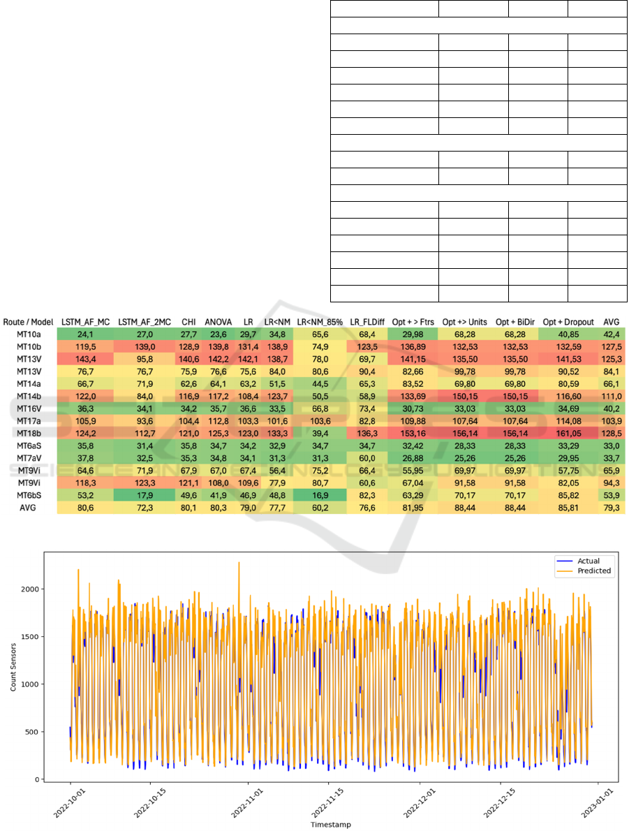
arrived at the results shown in Figure 1. As we can

see, the best results are obtained using the categorical

features determined by Linear Regression, only 4

numerical features. ('Count TomTom’, ‘85th

percentile Speed', 'IN_1' and 'Free Flow Speed Diff'),

optimized hyperparameters, the ‘85th Percentile

Speed’ as correlation index and a Simple LSTM

model. The results of this best model architecture can

be seen more clearly in Table 3, divided into three

groups of results: good, moderate and weak.

Table 3: Results best model architecture.

Route SMAPE MAE RMSE

Good Results

MT6b 16.94 13.90 18.30

MT7a 21.34 25.15 33.43

MT6a 34.71 33.89 42.87

MT18b 39.36 7.48 10.18

MT14a 44.46 70.06 10.91

MT14b 50.47 9.61 12.35

Moderate Results

MT10a 65.64 32.21 38.93

MT16 66.82 57.06 71.23

Weak Results

MT10b 74.89 72.74 77.65

MT9Carrubella 75.20 20.89 25.47

MT13Catania 78.04 13.29 18.87

MT13Cerza 80.59 29.06 38.53

MT9Catania 80.69 9.92 13.40

MT17a 103.56 70.27 83.96

Figure 1: Results of all model architectures.

Figure 2: MT6bSuperstradaCataniaPaterno prediction results.

DATA 2025 - 14th International Conference on Data Science, Technology and Applications

230

For this type of data, the results are classified as

follows: SMAPE less than 50% is considered good,

between 50% and 70% is considered moderate and

above 70% is considered poor. In this way, the

sensors were grouped into three categories, showing

that the model has different performances.

For certain routes, the model is able to predict the

actual traffic flows fairly well, demonstrating its

capability of learning sensor data patterns and scaling

the FCD data with reasonable accuracy, as shown in

Figure 2, which displays the predicted scaled data as

compared to the actual sensor counts for the route

MT6b (MT6bSuperstradaCataniaPaterno) which

achieved the best SMAPE value of 16.94. However,

as can be expected, the performance is not the same

for all sensors leading us to further analyse the route

differences.

8.5 Road Geometry Analysis

The results obtained with the final machine learning

model showed satisfactory performance on some

roads, while on others the performance was moderate

or unsatisfactory. Given this variation, we started an

analysis to investigate possible statistical or

geometric correlations between the characteristics of

the roads and the performance of the model.

We can begin our discussion with a more in-depth

analysis of the best performing sensor, the

MT6bSuperstradaCataniaPaterno, that is located in

one of the main extra-urban arterial roads linking

Catania with the western hinterland, facilitating the

movement of vehicles in a north-westerly direction,

for goods transport and commuting. The road section

consists of two separate carriageways with two lanes

in each direction. It is a high-capacity road with

significant traffic flows, mainly related to commuters

travelling between Catania and the surrounding areas.

Traffic flows tend to be higher in the morning and

evening, with possible slowdowns near the access

junctions to the Catania ring road.

The second-best performing sensor,

MT7aVialeLorenzoBolanocirconvallazione is also

on a dual carriageway, with two lanes in each

direction and, in some sections, a wide central traffic

divider separating the lanes and allowing good traffic

capacity.

Regarding the weaker results, such as those of the

sensors MT13ViaNuovaceloVersoCatania and

MT13ViaNuovaceloVersoCerza, it can be noted that

they are located on a road in the southern part of

Catania that crosses a predominantly residential and

commercial area, serving as a link between different

residential and industrial areas and facilitating access

to the city center. The road has a narrower cross-

section than the main urban arterials analysed so far,

with only one lane in each direction and large side

lay-bys for parking. The presence of frequent

intersections and side entrances reduces the flow

capacity in some sections, resulting in slower and

more discontinuous traffic.

Another weak result, the sensor

MT17aSS114VialeAfrica, located in the heart of city

center of Catania, is one of the main arteries

connecting the southern area to the city center, the

port area and the waterfront. It is characterized by

high traffic flows, with peaks at arrival and departure

times, influenced by commercial activities, public

transport stops and access to the city center and the

port. The road section of Viale Africa is wide, with

several lanes in each direction, with a central

reservation and wide pavements that facilitate

pedestrian movement. However, the presence of side

car parks and junctions contributes to increased

congestion during peak hours.

In such contexts, sudden peaks and decelerations

in traffic flow significantly reduce the accuracy of our

model’s estimates.

These results suggest that geometric

characteristics, such road typology and traffic flows,

play a fundamental role in the efficiency of the model

analyzed. Roads with a SMAPE below 50 are high-

capacity arterial roads with significant and stable

traffic flows. These roads present a relatively stable

penetration rate of FCD data (i.e. the percentage of

vehicles tracked by GPS technology in relation to the

total number of vehicles in transit), which allows for

a more accurate estimation of traffic flows, whereas a

low and variable penetration rate can limit the quality

and reliability of forecasts. This instability, combined

with factors such as frequent intersections, side

entrances, and parking areas, disrupts traffic patterns

and increases estimation errors. As a result, our

chosen model architecture performs significantly

better in structured, high-flow environments than on

roads with irregular or inconsistent traffic patterns.

9 CONCLUSIONS

The findings of this research indicate that the chosen

methodology for scaling FCD data on sensorless

roads has a promising performance, particularly on

high-capacity, constant-flow roads. The strategy

based on the LSTM model has proven to be effective

in identifying traffic patterns under certain

circumstances, allowing for more accurate estimates

of vehicle flow in sensorless regions.

In addition, a detailed study has shown that the

geometric and structural characteristics of the roads

have a significant impact on the performance of the

Scalable Trafﬁc Flow Estimation on Sensorless Roads Using LSTM and Floating Car Data

231

model. High-traffic arterial roads with constant

distribution have lower prediction errors, while roads

with large variations in FCD penetration rates,

frequent intersections and side parking are barriers to

the prediction accuracy using this type of approach.

A key point of this research is to validate of the

methodology’s ability to generate accurate

predictions using data derived from a single

correlated route, rather than relying on a larger group

of sensors for training. This has important

advantages, in terms of computational efficiency,

reduced complexity and a greater degree of

adaptation to the specifics of each route being

processed. This flexibility is critical for real-life

urban traffic management systems and helps their

implementation by enabling infrastructure-

constrained areas to improve the mobility monitoring

and planning strategies in a more accessible and

systematic way.

Based on these findings, the future work related

to this study can evaluate hybrid approaches that

enhance traffic prediction on more complex routes by

combining deep learning techniques with regular

models or other methods that are based on type of

road networks. In addition, it could be valuable to

develop a deeper investigation on the effects of FCD

data penetration, and potentially using other sensor

correlation techniques that may improve upon the

current results.

ACKNOWLEDGEMENTS

The work of Thamires de Souza Oliveira, David

Pagano and Salvatore Cavalieri, who contributed to

the development of the machine learning algorithm,

and Giovanni Calabrò, who was responsible for

downloading the data, has been supported by Italian

Ministry for Research (MUR) in the framework of

PNRR M4C2 Line 1.4, “National Centre for HPC,

Big Data and Quantum Computing”, Spoke 9 “Digital

Society & Smart Cities” (Code CN00000013, CUP

E63C22001000006). The work of Vincenza Torrisi,

who contributed to data collection and interpretation

of results analysis, has been supported by MUR in the

framework of PNRR project SAMOTHRACE,

(ECS00000022). Sensor data were provided by the

“ITS Laboratory” of the Department of Civil and

Architecture Engineering of Catania. Specifically, the

laboratory created within the project RE.S.E.T, is a

traffic monitoring, estimation and short-term

forecasting system, equipped with radar sensor and a

central control station for traffic data elaborations.

REFERENCES

Alkharusi, H. (2012). Categorical variables in regression

analysis: A comparison of dummy and effect coding.

International Journal of Education, 4(2), 202.

Almukhalfi, H., Noor, A., & Noor, T. H. (2024). Traffic

management approaches using machine learning and

deep learning techniques: A survey. Engineering

Applications of Artificial Intelligence, 133, 100164.

Berlotti, M., Di Grande, S., & Cavalieri, S. (2024). Proposal

of a Machine Learning Approach for Traffic. Sensors,

24(7), 2348.

Bernas, M., Płaczek, B., Korski, W., Loska, P., Smyła, J.,

& Szymała, P. (2018). A Survey and Comparison of

Low-Cost Sensing Technologies for Road Traffic

Monitoring. Sensors, 18(10), 3243. https://doi.org/

10.3390/s18103243

CATANIATODAY. (2024). Classifica sulla qualità della

vita, Catania risale: è 83esima su 107. Retrieved from

https://www.cataniatoday.it/cronaca/classifica-qualita-

della-vita-catania-2024.html.

Chen, C., Twycross, J., & Garibaldi, J. M. (2017). A new

accuracy measure based on bounded relative error for

time series forecasting. PLoS One, 12(3), e0174202.

Dai, G., Ma, C., & Xu, X. (2019). Short-Term Traffic Flow

Prediction Method for Urban Road Sections Based on

Space–Time Analysis and GRU. IEEE Access, 7,

143025-143035. https://doi.org/10.1109/ACCESS.201

9.2941280

Dash, C. S. K., Behera, A. K., Dehuri, S., & Ghosh, A.

(2023). An outlier’s detection and elimination

framework in classification task of data mining.

Decision Analytics Journal, 6, 100164. https://doi.

org/10.1016/j.dajour.2023.100164

De Fabritiis, C., Ragona, R., & Valenti, G. (2008, October).

Traffic estimation and prediction based on real-time

floating car data. In 2008 11th International IEEE

Conference on Intelligent Transportation Systems (pp.

197-203). IEEE.

Duan, Y., Lv, Y., & Wang, F.-Y. (2016). Travel time

prediction with LSTM neural network. 2016 IEEE 19th

International Conference on Intelligent Transportation

Systems (ITSC). https://doi.org/10.1109/ITSC.2016

.7795686

Gomes, B., Coelho, J., & Aidos, H. (2023). A survey on

traffic flow prediction and classification. Intelligent

Systems with Applications, 20, 200268.

https://doi.org/10.1016/j.iswa.2023.200268

Hodson, T. O. (2022). Root-mean-square error (RMSE) or

mean absolute error (MAE): when to use them or not.

Geoscientific Model Development, 15, 5481-5487.

Houbraken, M., Logghe, S., Audenaert, P., Colle, D., &

Pickavet, M. (2018). Examining the potential of

floating car data for dynamic traffic management. IET

Intelligent Transport Systems, 12(5), 335–344.

https://doi.org/10.1049/iet-its.2016.0230

Jaeger, T. F. (2008). Categorical Data Analysis: Away from

ANOVAs (transformation or not) and towards Logit

Mixed Models. Journal of Memory and Language,

59(4), 434-446.

DATA 2025 - 14th International Conference on Data Science, Technology and Applications

232

Jabbar, H. K. (2015). Methods to avoid overfitting and

underfitting in supervised machine learning

(comparative study). University of Misan, Misan, Iraq,

and Department of Computer Science, Aligarh Muslim

University, Aligarh, India. Retrieved from https://www.

jmail.com.

Kang, D., Yisheng, L., & Chen, Y. Y. (2017). Short-term

traffic flow prediction with LSTM recurrent neural

network. IEEE 19th International Conference on

Intelligent Transportation Systems (ITSC). https://doi.

org/10.1109/ITSC2017.8317872

Kent State University Libraries. (2018). SPSS Statistics

Tutorials and Resources. Retrieved from https://

libguides.library.kent.edu/SPSS.

Keras: Deep Learning for humans. Retrieved from

https://keras.io/.

Kim, J., Oh, S., Kim, H., & Choi, W. (2023). Tutorial on

time series prediction using 1D-CNN and BiLSTM: A

case example of peak electricity demand and system

marginal price prediction. Proceedings of Engineering

Applications of AI, Article 106817. https://doi.

org/10.1016/j.engappai.2023.106817

Kohonen, T. (1972). Correlation matrix memories. IEEE

Transactions on Computers, 100(4), 353-359.

La Greca, P., & Martinico, F. (2018). Shaping the

Sustainable Urban Mobility: The Catania Case Study.

In R. Papa, R. Fistola, & C. Gargiulo (Eds.), Smart

Planning: Sustainability and Mobility in the Age of

Change (pp. 359-374). Springer.

Meiying, Q., Xiaoping, M., Jianyi, L., & Ying, W. (2011).

Time-series gas prediction model using LS-SVR within

a Bayesian framework. Mining Science and

Technology, 21(1), 153-157.

Mystakidis, A., Koukaras, P., & Tjortjis, C. (2025).

Advances in Traffic Congestion Prediction: An

Overview of Emerging Techniques and Methods. Smart

Cities, 8(1), 25. https://doi.org/10.3390/smartcities8

010025

Pandey, R., Khatri, S. K., Singh, N. K., & Verma, P. (Eds.).

(2022). Artificial intelligence and machine learning for

EDGE computing. Academic Press.

https://doi.org/10.1016/C2020-0-01569-0

Peng, Y.-L., & Lee, W.-P. (2024). Practical guidelines for

resolving the loss divergence caused by the root-mean-

squared propagation optimizer. Applied Soft

Computing, 153, 111335. https://doi.org/10.1016/

j.asoc.2022.111335

Rana, R., & Singhal, R. (2015). Chi-square test and its

application in hypothesis testing. Journal of the Practice

of Cardiovascular Sciences, 1(1), 69–71.

https://doi.org/10.4103/2395-5414.157577

Rodríguez, P., Bautista, M. A., Gonzàlez, J., & Escalera, S.

(2018). Beyond one-hot encoding: Lower dimensional

target embedding. Image and Vision Computing, 75,

21-31. https://doi.org/10.1016/j.imavis.2018.04.002

scikit-learn: Machine Learning in Python. Retrieved from

https://scikit-learn.org/stable/index.html.

Sedgwick, P. (2012). Pearson’s correlation coefficient.

BMJ, 345, e4483. https://doi.org/10.1136/bmj.e4483

TensorFlow: An end-to-end platform for machine learning.

Retrieved from https://www.tensorflow.org/.

Tato, A., & Nkambou, R. (2018). Improving Adam

optimizer. Workshop track - ICLR 2018, Department of

Computer Science, Université du Québec à Montréal,

Montréal, Quebec, Canada.

TomTom Move. Retrieved from https://move.tom

tom.com/.

Torrisi, V., Ignaccolo, M., & Inturri, G. (2018). Innovative

Transport Systems to Promote Sustainable Mobility:

Developing the Model Architecture of a Traffic Control

and Supervisor System. In Proceedings of

Computational Science and Its Applications–ICCSA

2018: 18th International Conference (pp. 622-637).

Springer.

Tu, Y., Lin, S., Qiao, J., et al. (2021). Deep traffic

congestion prediction model based on road segment

grouping. Applied Intelligence, 51, 8519–8541.

https://doi.org/10.1007/s10489-020-02152-x

Vázquez, J. J., Arjona, J., Linares, M. P., & Casanovas-

Garcia, J. (2020). A Comparison of Deep Learning

Methods for Urban Traffic Forecasting using Floating

Car Data. Transportation Research Procedia, 47, 195-

202. https://doi.org/10.1016/j.trpro.2020.03.079

Wang, Y., Ke, S., An, C., Lu, Z., & Xia, J. (2024). A Hybrid

Framework Combining LSTM NN and BNN for Short-

term Traffic Flow Prediction and Uncertainty

Quantification. KSCE Journal of Civil Engineering, 28

(1),363-374. https://doi.org/10.1007/s12205-023-2457-y

Wang, J.-D., Noto Susanto, C. O., & Oktomy, C. (2023).

Traffic Flow Prediction with Heterogeneous Data Using

a Hybrid CNN-LSTM Model. Computers, Materials and

Continua, 76(3), 3097-3112. https://doi.org/10.32604/

cmc.2023.040914

Wu, H., & Gu, X. (2015). Towards dropout training for

convolutional neural networks. Neural Networks, 71, 1–

10. https://doi.org/10.1016/j.neunet.2015.07.003

Yu, Y., Si, X., Hu, C., & Zhang, J. (2019). A review of

recurrent neural networks: LSTM cells and network

architectures. Neural Computation, 31(7), 1235–1270.

https://doi.org/10.1162/neco_a_01199

Scalable Trafﬁc Flow Estimation on Sensorless Roads Using LSTM and Floating Car Data

233