Estimation of Vehicle States Using a Cascaded Hybrid Estimation
Method
Marvin Glomsda
a
, Hendrik Tino Prümer
b
and Philipp Maximilian Sieberg
c
Chair of Mechatronics, University of Duisburg-Essen, Lotharstr. 1, Duisburg, Germany
Keywords: Hybrid State Estimation, Hybrid Estimation Methods, Cascaded Hybrid Estimation Method, Vehicle State
Estimation.
Abstract: Three models using a cascaded hybrid estimation method with physical models of different degrees of
accuracy are evaluated for their overall precision and interpretability. Hybrid estimation methods hereby
denote methods concatenating the properties of physics-based models and artificial neural networks for the
purpose of improved state estimation. Cascaded hybrid estimation methods are a subtype of these methods,
combining a physical model and an artificial neural network in a way that one acts as the input of the other.
In this publication the result of a physical model is fed into a neural network to improve the estimation quality.
It can be shown that the degree of accuracy of the physical model has an influence on the overall estimation
quality, with more accurate physical models yielding better results, but less accurate models can provide a
more significant improvement through the artificial neural network. This is likely due to the larger residual
error that can be used to train the artificial neural network.
1 INTRODUCTION
The requirements for vehicle state estimation
continue to rise. Therefore, new approaches, so-called
hybrid methods, have been developed, that combine
a physics-based model with an artificial neural
network (Sieberg et al., 2019). As the development of
artificial neural networks and such hybrid methods
continues, it is important to examine different
approaches. Various methods, shown in (Gräber et
al., 2018; Kim et al., 2021; Li et al., 2021; Wu et al.,
2024), could be interpreted as cascaded hybrid
estimation models, which thus far has not been
extensively tested for vehicle dynamics. The
information flow and the decision-making of artificial
neural networks tends to be non-transparent, as their
structure tends to be complex, especially for
demanding estimation tasks. This could also be the
case with a cascaded hybrid method, as all
information is passed through the artificial neural
network. The EU Artificial Intelligence Act (Smuha,
2025) shows that the first legal requirements are
already being placed on artificial neural networks and
a
https://orcid.org/0009-0003-2821-0253
b
https://orcid.org/0009-0007-2349-6474
c
https://orcid.org/0000-0002-4017-1352
their operation. The interpretability and therefore
traceability of the decision-making of an artificial
neural network are also regulated. Security,
reliability, transparency, traceability, and
documentation are focussed and various operators are
held responsible to ensure these aspects (Smuha,
2025). Interpretation methods are necessary for
transparency and traceability. Some of these methods
are listed in (Carvalho et al., 2019; Linardatos et al.,
2020; Zhang et al., 2021), and offer options for
interpreting artificial neural networks.
2 METHODOLOGY
This publication aims to investigate if cascaded
hybrid estimation models offer an attractive
opportunity to enhance state estimation based solely
on physical modelling. To validate this approach,
physical models with three different degrees of
accuracy are used and combined with a subsequent
artificial neural network. All three estimation tasks
are chosen from the automotive field, however the
126
Glomsda, M., Prümer, H. T. and Sieberg, P. M.
Estimation of Vehicle States Using a Cascaded Hybrid Estimation Method.
DOI: 10.5220/0013646200003970
In Proceedings of the 15th International Conference on Simulation and Modeling Methodologies, Technologies and Applications (SIMULTECH 2025), pages 126-134
ISBN: 978-989-758-759-7; ISSN: 2184-2841
Copyright © 2025 by Paper published under CC license (CC BY-NC-ND 4.0)

findings from the investigation should be applicable
over a wide variety of application fields. For the
estimation tasks within this publication a simulation
environment is used, which combines IPG CarMaker
and MATLAB & Simulink in a co-simulation. The
application examples chosen for this investigation are
the estimation of the side-slip angle, the yaw rate, and
the tyre load of the front left tyre. For proper
investigation, the degree of accuracy was varied for
the physical models utilised for each state estimation.
Table 1 gives an overview over the physical models
used and their respective degree of accuracy.
Table 1: Overview of degree of accuracy for chosen state
estimation parameters, derived from (Schramm et al.,
2018).
Parameter Physical Model Degree of
Accurac
y
Side-slip
an
g
le
Double-track model High
Yaw rate Equilibrium of
momentum of double-
trac
k
model
Medium
Tyre load
(
front left
)
Quarter-vehicle model Low
By using models with different accuracy, it can be
investigated if the estimation quality can be increased
by cascading physical models with a subsequent
artificial neural network. To assess the quality of the
output, three main performance indices are used, root
mean square error, permutation feature importance,
and local interpretable model-agnostic explanation.
The root mean square error takes into account the
ground truth of IPG CarMaker. Permutation feature
importance and local interpretable model-agnostic
explanation, on the other hand, serve to evaluate how
interpretable the state estimation is. The permutation
feature importance is a measure for global
interpretability (Molnar, 2020), while the local
interpretable model-agnostic does the same locally
(Ribeiro et al., 2016). This is based on the concern of
having all information processed through the artificial
neural network and the estimated state using no
measured quantity directly. To evaluate how
beneficial the integration of the artificial neural
network within the hybrid method is to the overall
state estimation, the output of each physical model is
evaluated as well.
3 MODELLING
In this section, the used methods will be described.
First, the overall structure will be presented, followed
by its subparts, namely the three different physical
models and the artificial neural network. Lastly, the
driving manoeuvres, used to generate the data for the
training of the artificial neural network and the
overall validation, will be presented.
3.1 Overall Structure
As described in the Methodology section, a cascaded
hybrid state estimation approach shall be used for this
study. This approach is implemented for each
estimated parameter individually. The basic structure
of the artificial neural network remains unchanged for
the different estimation tasks. The applied physical
models are presented in Table 1. The IPG CarMaker
environment, a multi-body vehicle simulation
validated for example by (Cheok et al., 2023),
provides the input data into the models as well as the
ground truth values for the estimation tasks. The
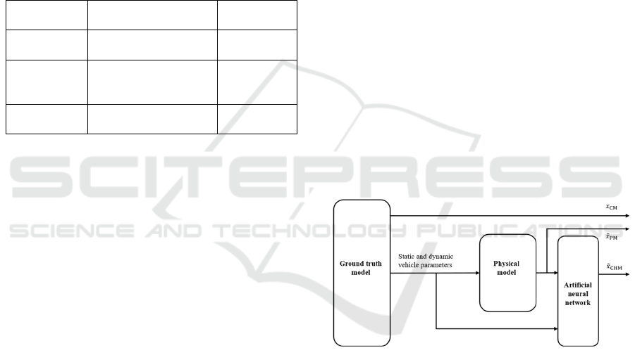
overall structure is depicted in Figure 1. IPG
Carmaker provides sensor signals, which are used as
inputs into the physical model as well as the artificial
neural network for estimating the target quantities.
These estimations are then compared to the ground
truth quantities, which are also provided by IPG
Carmaker. Thus, the estimation of the physical model
can be compared against the estimation by the hybrid
method.
Figure 1: Overall structure of the simulation environment.
3.2 Model for Side-Slip Angle
Estimation
A twin-track model as described in (Schramm et al.,
2018) is used as the basis for the physical model that
estimates the side-slip angle. All necessary arguments
for this model are taken from the IPG CarMaker
environment, except for the vehicle velocity, the
acceleration as well as the side-slip angle and its
derivative. These quantities are representing inner
states of the physical model. Vehicle acceleration and
side-slip angle derivative are both integrated and the
fed back to the system, respectively. Both values are
initialised with zero, as the vehicle starts each
Estimation of Vehicle States Using a Cascaded Hybrid Estimation Method
127

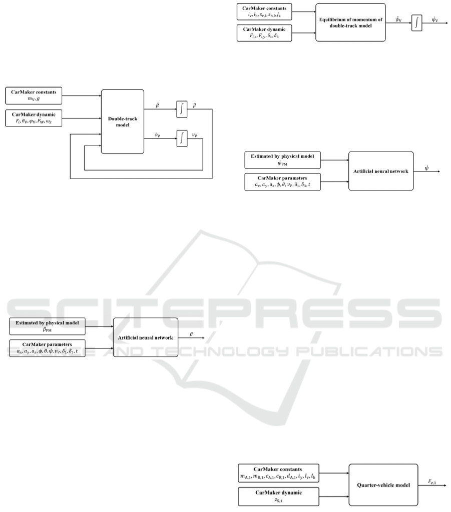
simulation run in straight standstill. Constants are the
vehicle mass and gravitational acceleration. In
contrast the chassis forces for each suspended wheel,
the vehicle roll and pitch angle, the wind force acting
on the entire vehicle, and the tyre velocities are
dynamic input quantities provided by IPG CarMaker.
Figure 2 depicts this approach.
Figure 2: Implementation of the physical model for side-
slip angle estimation.
The side-slip angle 𝛽 is used as the single output
of the twin-track model and fed into the artificial
neural network alongside longitudinal, lateral, and
vertical acceleration, roll, pitch, and yaw angle,
vehicle velocity, steering angle of the front wheels,
and the simulated time. This is depicted in Figure 3.
The structure of the artificial neural network will be
described in section 3.5.
Figure 3: Implementation of the artificial neural network for
side-slip angle estimation.
3.3 Model for Yaw Rate Estimation
As the degree of accuracy for the yaw rate estimation
shall be lower compared to the task of estimating the
side-slip angle, the momentum equilibrium of the
twin-track model is selected for this purpose instead
of the direct use of the twin-track model. The time
integration needed for the calculation of the yaw rate
with this approach leads to a summation of the
integration error, as the yaw rate is not fed back into
the model. The chassis forces for each suspended
wheel and the steering angle for both front wheels
serve as the dynamic inputs for this model, while
wheelbase, the longitudinal position of the centre of
gravity, front and rear track width and the moment of
inertia of the vehicle are constant. This structure is
visualised in Figure 4.
Figure 4: Implementation of the physical model for yaw
rate estimation.
As shown in Figure 5, the artificial neural network
for the estimation of the yaw rate uses the same inputs
from IPG CarMaker as the one for the side-slip angle
estimation. In addition, the physical model provides
the estimation of the yaw rate as an input.
Figure 5: Implementation of the artificial neural network for
yaw rate estimation.
3.4 Model for Tyre Load Estimation
For the estimation of the tyre load, a quarter-car
model is used for the physical part of the hybrid
estimation. This model can be represented by a linear
state-space representation. The structure of the
quarter-car model is based on the equations from
(Schramm et al., 2018). The constants such as tyre
stiffness, spring and damper constants, tyre mass and
body mass of the front left vehicle body are taken
from the IPG CarMaker environment, as shown in
Figure 6. The damping of the tyre is assumed to be
zero. Other constants used for this estimation are the
inertia of rotation around the tyre’s rotation axis and
the distances to the vehicle's centre of gravity. The
excitation caused by the road surface is dynamically
provided by the IPG CarMaker environment for the
contact point of the front left tyre and fed to the
system.
Figure 6: Implementation of the physical model for tyre
load estimation.
Alongside the estimated tyre load of the front left
tyre, the artificial neural network is given
longitudinal, lateral, and vertical acceleration, pitch
angle, road excitation, simulated time, and the lengths
of spring, damper, and distance of wheel carrier to
SIMULTECH 2025 - 15th International Conference on Simulation and Modeling Methodologies, Technologies and Applications
128

centre of gravity of the front left as well as the rear
left tyre, as depicted in Figure 7.
Figure 7: Implementation of the artificial neural network for
tyre load estimation.
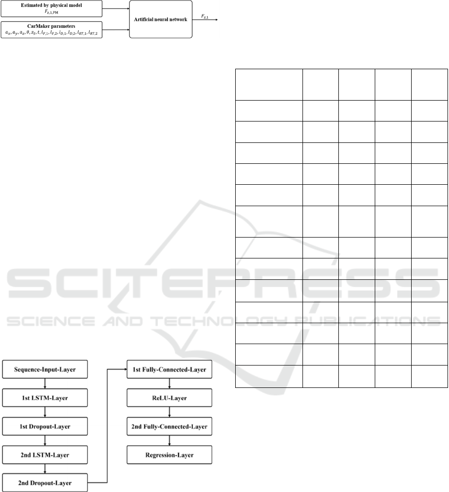
3.5 Structure of Artificial Neural
Network
An identical base structure was chosen for the
artificial neural networks of all three estimation
models. As the deviation between the outputs of each
physical and the ground truth model may incorporate
nonlinearities and represents a time-series prediction
problem, an artificial neural network based on long
short-term memory (LSTM) cells was chosen. (Zhang
et al., 2024) showed that such networks can be used
for the modelling of vehicle dynamics.
The concrete network structure used for this study
is shown in Figure 8 and starts with a sequence input
layer that feeds the time series data to two LSTM
layers. To omit overfitting issues, a dropout layer is
integrated after each LSTM layer, deactivating LSTM
cells randomly during the training process. Lastly, the
information passes through one fully-connected
layer, one rectified linear unit layer, and one single
fully-connected termination neuron, as only one
parameter is to be estimated by each artificial neural
network. A regression layer is added to allow a
continuous estimation.
Figure 8: Structure of the artificial neural network used for
all three models presented in this publication.
Of the generated training data, 70 % are used for
the training of the artificial neural network itself,
while the other 30 % are used for in-training
validation. The data are based on the simulations of
the driving manoeuvres presented in section 3.6. No
experimental data were used to train the models.
A hyperparameter optimisation was carried out
for each artificial neural network individually. The
results of this hyperparameter optimisation are shown
in Table 2 for all three artificial neural networks.
Table 2: Results of hyperparameter optimisation.
Hyper-
parameter
Range Side-
Slip
An
g
le
Yaw
Rate
Tyre
Load
Sequence
length
50 –
200
137 170 184
Hidden layers
(LSTM 1)
32 –
128
122 83 124
Dropout 1 0.1 –
0.5
0.1088 0.4454 0.3965
Hidden layers
(LSTM 2)
32 –
128
110 106 120
Dropout 2 0.1 –
0.5
0.3164 0.2441 0.4834
Neurons of
fully connected
laye
r
1
10 –
100
61 19 16
Batch size 50 –
200
90 53 69
Gradient
threshol
d
0.5 – 5 1.9771 1.6865 4.4373
Initial learning
rate
10
-2
–
10
-4
0.0028 0.0060 0.0041
Learning rate
drop
p
erio
d
5 –
50
44 33 22
Learning rate
dro
p
facto
r
0.1 –
0.9
0.1887 0.4875 0.6515
Validation
frequenc
y
50 –
200
151 117 55
L2
regularisation
10
-2
–
10
-6
1.7509
∙10
-6
1.8262
∙10
-6
1.2816
∙10
-6
For this purpose, the sequence length of the input
and the LSTM network configuration, such as the size
of the hidden layer, fully connected layer, and the
values of the dropout layer are chosen as
hyperparameters. The Adam optimizer is used for this
purpose. The number of epochs is limited to 50 for
the Bayesian optimisation method (Frazier, 2018).
Furthermore, the batch size, gradient threshold, initial
learning rate, learning rate drop period, learning rate
drop factor, validation frequency (with validation
patience of 100), and the use of L2 regularisation are
defined as hyperparameters. The hyperparameters for
the three neural networks are approximated after 30
iterative steps of the Bayesian optimisation method
with the search for the lowest root mean square error
of the normalised validation data. The results of this
optimisation do not use the minimum or maximum
Estimation of Vehicle States Using a Cascaded Hybrid Estimation Method
129

values of the specified intervals. L2 regularisation is
required for each neural network presented here.
3.6 Manoeuvres for Data Generation
According to the estimation tasks, the same
manoeuvres were used to obtain the data used to train,
validate, and test the hybrid estimation of the side-slip
angle and the yaw rate. For those manoeuvres,
attention was paid to high excitation of the estimation
quantities. Two different slaloms and one double lane
change setup were used here with multiple velocities
used for all of them. Table 3 gives an overview over
the exact manoeuvre setups. All simulation outputs
were updated every 0.01 s for the duration of the
manoeuvres. The measure given for each slalom
determines the distance between consecutive cones of
the slalom. The double lane change used for training
data generation was the one from the General German
Automobile Club (ADAC) (Diehm et al., 2013),
while the double lane change according to ISO
3888-1 (Standardization, 2018) with an entry velocity
of 90 km/h was used to generate the test data for the
estimation of side-slip angle and yaw rate, which is
listed in Table 4.
Table 3: Overview of all manoeuvres used for training data
generation in this study.
Manoeuvre Variable Range Interval
Side-slip angle and yaw rate estimation
Slalom 18 m Velocity 20 - 60
km/h
20 km/h
Slalom 36 m Velocity 20 - 100
km/h
20 km/h
Double lane
chan
g
e
(
ADAC
)
Velocity 20 - 100
km/h
20 km/h
Tyre load estimation
Speed bump Velocity 5 - 11
km/h
2 km/h
Bump
height
0 - 8 cm 2 cm
To generate the training data for the tyre load
estimation, a speed bump setup with three subsequent
speed bumps of equal height was used. Vehicle
velocity and height of the bumps were varied
according to Table 3.
The test data in this case was obtained with a track
consisting of three bumps of different height and a
vehicle velocity of 6 km/h. The heights of the bumps
were set to 1 cm for the first, 7 cm for the second, and
5 cm for the third bump. Table 4 shows the setups
used for test data generation.
Table 4: Overview of the manoeuvres used for test data
generation in this study.
Manoeuvre Variable Value
Side-slip angle and yaw rate estimation
Double lane
change (ISO)
Entry
velocit
y
90 km/h
Tyre load estimation
Speed bump Velocity 6 km/h
Bump height 1 cm (first bump)
7 cm (second bump)
5 cm (thir
d
b
ump)
These relatively simple manoeuvres were chosen
on purpose to enable potential reasoning within the
interpretability part of each estimation evaluation.
4 RESULTS
In this section, the results achieved by the hybrid
method for the different estimation tasks will be
presented. The structure follows the sequence
established in Table 1, starting with the results for the
side-slip angle estimation, followed by the results for
the yaw rate estimation, and completed by the results
for the estimation of the tyre load. Each estimation
approach is discussed individually here, as a
comparative conclusion follows in the next section.
4.1 Results for Side-Slip Angle
Estimation
First of all, a visual comparison is presented in Figure
9. As it can be seen in this figure, the direct output of
the physical model matches the ground truth curve
better than the output of the artificial neural network
that was supposed to correct any remaining deviations
and increase the accuracy.
This can also be seen in the root mean square error
that calculates to 0.0004 for the output of the physical
model and to 0.0023 for the output of the artificial
neural network.
Figure 9: Visual comparison between ground truth (red),
physical model (blue) and cascaded hybrid state estimation
(green) for side-slip angle estimation.
SIMULTECH 2025 - 15th International Conference on Simulation and Modeling Methodologies, Technologies and Applications
130

The permutation feature importance yields a very
conclusive result for the artificial neural network used
as part of the cascaded hybrid state estimation for the
estimation of the side-slip angle. The artificial neural
network relies nearly entirely on the estimated side-
slip angle provided by the physical model. However,
the slight impact of the other inputs seems to worsen
the estimation instead of improving it. Table 5 shows
the permutation feature importance for all inputs of
this artificial neural network.
Table 5: Permutation feature importance for artificial neural
network used for side-slip angle estimation.
Feature Relative Importance
𝛽

199.2931 %
𝑎

0.6652 %
𝑎

0.6643 %
𝜃

0.6259 %
𝜙

0.3648 %
𝛿

0.3200 %
𝛿

0.2561 %
𝑣

0.0098 %
𝜓

0.0040 %
𝑡
-0.0054 %
𝑎

-0.2826 %
This assumption can be supported by the local
interpretable model-agnostic explanation which was
assessed exemplarily for the deviation highlighted on
the left side of Figure 9. This analysis shows that at
that exact deviation the calculation of the artificial
neural network was dominated by the yaw rate among
other inputs while the estimation of the physical
model was completely neglected in this moment, as
can be seen in Table 6.
Table 6: Local interpretable model-agnostic explanation for
the left deviation highlighted in Figure 9.
Feature Model Coefficient
𝜓

0.0023
𝜃

0.0012
𝑎

0.0012
𝛿

0.0011
𝛿

0.0011
𝑎

0.0008
𝜙

0.0007
𝑎

0.0007
𝑡
0.0000
𝑣

0.0000
𝛽

0.0000
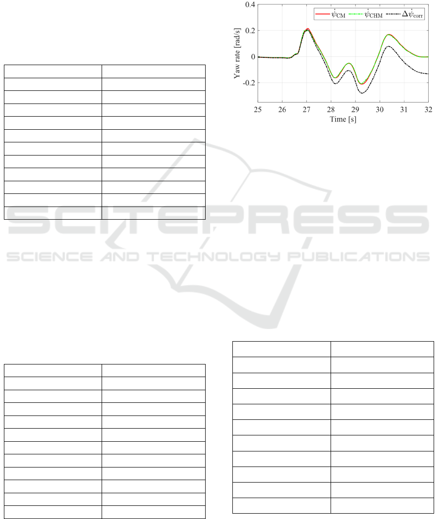
4.2 Results for Yaw Rate Estimation
Figure 10 shows the great influence of the integration
error obtained when using the physical model
described in subsection 3.3 without any correction.
The output of the physical model was corrected for a
static offset.
Figure 10: Estimated yaw rate for test data: Ground truth
model (red), estimation by the physical model (black,
corrected for static offset) and by cascaded hybrid state
estimation (green) for yaw rate estimation.
This drastic improvement is also supported by the
root mean square error, which is 0.0657 for the
physical model after the offset correction and 0.0041
for the output of the artificial neural network on the
test data, more than one order of magnitude better.
The permutation feature importance is much more
balanced for the yaw rate estimation compared to the
side-slip angle estimation. Longitudinal acceleration
has the highest importance, followed by the roll
angle. The results for all inputs can be seen in Table
7.
Table 7: Permutation feature importance for artificial neural
network used for yaw rate estimation.
Feature Relative Importance
𝑎

88.8793 %
𝜃

56.1443 %
𝑎

20.0293 %
𝜙

13.1013 %
𝛿

8.0284 %
𝛿

6.4708 %
𝑣

0.7281 %
𝑡
-0.0033 %
𝜓


-0.2019 %
𝑎

-8.8256 %
Estimation of Vehicle States Using a Cascaded Hybrid Estimation Method
131

As no large deviations can be observed, the local
interpretable model-agnostic explanation, performed
on the first peak visible in Figure 10, yields similar
results as the permutation feature importance. These
results are shown in Table 8.
Table 8: Local interpretable model-agnostic explanation for
first peak visible in Figure 10.
Feature Model Coefficient
𝑎

0.0205
𝜃

0.0156
𝜙

0.0145
𝑎

0.0141
𝛿

0.0117
𝑎

0.0116
𝛿

0.0104
𝜓


0.0008
𝑡
0.0000
𝑣

0.0000
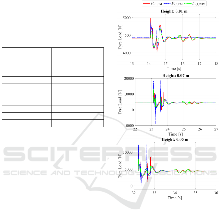
4.3 Results for Tyre Load Estimation
For a proper visual examination, Figure 11 shows
each bump of the test manoeuvre separately. At the
excitations at about 14 s, 23 s, and 32 s, the direct
effect of each bump can be seen, while at the
excitations at about 16 s, 25 s, and 34 s, the effect of
the rear wheel hitting the same bump is visible. It
becomes apparent that the quarter-car model is unable
to replicate these second excitations. The cascaded
hybrid state estimation, while being worse at the
estimation of the exact values of the single peaks, can
replicate the effect caused by the rear wheel.
When looking at the root mean square error, this
results in an improvement from 0.0389 for the
physical model to 0.0174 for the output of the
artificial neural network.
The permutation feature importance shows the
highest influence for the vertical acceleration of the
vehicle, followed by the elevation of the vehicle’s
centre of gravity, the estimated tyre load of the
physical model and the length of the wheel carrier of
the rear left wheel. Table 9 shows the permutation
feature importance of all inputs of the artificial neural
network used for tyre load estimation of the front left
tyre.
Figure 11: Estimated tyre load for front left wheel: Ground
truth model (red), estimation by the physical model (blue)
and by cascaded hybrid state estimation (green), portrayed
separately for each bump of the test manoeuvre.
The local interpretable model-agnostic
explanation, calculated for the first peak portrayed in
Figure 11, shows a similar result as the permutation
feature importance for this model, with an even
higher reliance on the estimated tyre load of the
physical model. All results of this evaluation are
shown in Table 10.
SIMULTECH 2025 - 15th International Conference on Simulation and Modeling Methodologies, Technologies and Applications
132

Table 9: Permutation feature importance for artificial neural
network used for tyre load estimation of front left tyre.
Feature Relative Importance
𝑎

335.9293 %
𝑧

149.7106 %
𝐹
,,
93.0265 %
𝑙
,
63.9848 %
𝑎

23.8769 %
𝑙
,
19.2051 %
𝑙
,
14.9819 %
𝜃

13.2897 %
𝑙
,
10.9508 %
𝑣

3.6284 %
𝑙
,
3.1289 %
𝑙
,
1.6099 %
𝑎

0.5285 %
𝑡
-0.0026 %
Table 10: Local interpretable model-agnostic explanation
for first peak shown in Figure 11.
Feature Model Coefficient
𝐹
,,
93.7598
𝑎

61.6276
𝑧

48.2679
𝑣

44.3520
𝑎

31.3720
𝑙
,
7.9202
𝑡
6.5219
𝑙
,
5.7612
𝑎

0.0000
𝜃

0.0000
𝑙
,
0.0000
𝑙
,
0.0000
𝑙
,
0.0000
𝑙
,
0.0000
5 CONCLUSION
The results for the root mean square error are
ambiguous, as Table 11 shows. For the side-slip angle
estimation, the root mean squared error increases for
the hybrid method compared to the sole use of the
physical model, but at a very low level compared to
the other two estimation tasks. Yaw rate and tyre load
estimation show an improvement in estimation
quality.
Table 11: Overview of root mean square error for chosen
state estimation parameters.
Parameter Physical Model Cascaded
Hybrid State
Estimation
Side-slip angle 0.0004 0.0023
Yaw rate 0.0657 0.0041
T
y
re loa
d
0.0389 0.0174
The permutation feature importance shows a
different dependency of the artificial neural networks
on the parameters estimated by the physical models.
While the artificial neural network for the estimation
of the side-slip angle relies nearly completely on this
input, the artificial neural network used for the
estimation of the yaw rate near-completely omits the
use of the input provided by the physical model. The
artificial neural network of the model estimating the
tyre load uses the value estimated by the connected
physical model as one of the most important inputs,
while also relying strongly on some of the other
inputs provided.
These findings lead to the conclusion that the
artificial neural network as part of a cascaded hybrid
state estimation needs a certain room for improving
the estimation to be able to train properly. This is an
interesting finding as normalised values were used for
the training of the artificial neural networks. But it is
reasonable to assume that the small deviation
remaining after the physical model for the side-slip
angle estimation might have been incidental rather
than being related to any of the other inputs provided
to the artificial neural network in this specific case.
6 OUTLOOK
One evaluation parameter currently not analysed, is
the computational effort needed to carry out the
cascaded hybrid state estimation models. This could
be achieved by comparing the effect of the different
simulation stages (ground truth model, with added
physical model, and with added cascaded hybrid
method) on the central processing unit. The cascaded
hybrid models obtained in this study should also be
tested with more difficult test manoeuvres on their
robustness. Lastly, a comparison to other (hybrid)
state estimation methods, including Kalman filter
based methods, should be undertaken to find the
optimal structure for a given estimation task.
The original contributions presented in this study
are included in the article. Further inquiries can be
directed to the corresponding author.
Estimation of Vehicle States Using a Cascaded Hybrid Estimation Method
133

REFERENCES
Carvalho, D. V., Pereira, E. M., & Cardoso, J. S. (2019).
Machine learning interpretability: A survey on methods
and metrics. Electronics, 8(8), 832.
Cheok, J. H., Lee, K. O., Aparow, V. R., Amer, N., Peter,
C., & Magaswaran, K. (2023). Validation of scenario-
based virtual safety testing using low-cost sensor-based
instrumented vehicle. Journal of Mechanical
Engineering and Sciences, 9520-9541.
Diehm, G., Maier, S., Flad, M., & Hohmann, S. (2013).
Online identification of individual driver steering
behaviour and experimental results. 2013 ieee
international conference on systems, man, and
cybernetics,
Frazier, P. I. (2018). Bayesian optimization. In Recent
advances in optimization and modeling of
contemporary problems (pp. 255-278). Informs.
Gräber, T., Lupberger, S., Unterreiner, M., & Schramm, D.
(2018). A hybrid approach to side-slip angle estimation
with recurrent neural networks and kinematic vehicle
models. IEEE Transactions on Intelligent Vehicles,
4(1), 39-47.
Kim, D., Kim, G., Choi, S., & Huh, K. (2021). An
integrated deep ensemble-unscented Kalman filter for
sideslip angle estimation with sensor filtering network.
IEEE Access, 9, 149681-149689.
Li, W., Zhang, J., Ringbeck, F., Jöst, D., Zhang, L., Wei,
Z., & Sauer, D. U. (2021). Physics-informed neural
networks for electrode-level state estimation in lithium-
ion batteries. Journal of Power Sources, 506, 230034.
Linardatos, P., Papastefanopoulos, V., & Kotsiantis, S.
(2020). Explainable ai: A review of machine learning
interpretability methods. Entropy, 23(1), 18.
Molnar, C. (2020). Interpretable machine learning. Lulu.
com.
Ribeiro, M. T., Singh, S., & Guestrin, C. (2016). " Why
should i trust you?" Explaining the predictions of any
classifier. Proceedings of the 22nd ACM SIGKDD
international conference on knowledge discovery and
data mining,
Schramm, D., Hiller, M., & Bardini, R. (2018). Vehicle
dynamics. Modeling and Simulation. Berlin,
Heidelberg, 2nd Edition.
Sieberg, P. M., Blume, S., Harnack, N., Maas, N., &
Schramm, D. (2019). Hybrid state estimation
combining artificial neural network and physical
model. 2019 IEEE Intelligent Transportation Systems
Conference (ITSC),
Smuha, N. A. (2025). Regulation 2024/1689 of the Eur.
Parl. & Council of June 13, 2024 (Eu Artificial
Intelligence Act). International Legal Materials, 1-148.
Standardization, I. O. f. (2018). ISO 3888 ‐ 1: 2018
Passenger cars—Test track for a severe lane‐change
manoeuvre—Part 1: Double lane‐change. In.
Wu, M., Wang, Y., Zhang, Y., & Li, Z. (2024). Physics-
Informed Neural Network for Mining Truck
Suspension Parameters Identification. Advanced
Vehicle Control Symposium,
Zhang, Y., Huang, Y., Deng, K., Shi, B., Wang, X., Li, L.,
& Song, J. (2024). Vehicle Dynamics Estimator
Utilizing LSTM-Ensembled Adaptive Kalman Filter.
IEEE Transactions on Industrial Electronics.
Zhang, Y., Tiňo, P., Leonardis, A., & Tang, K. (2021). A
survey on neural network interpretability. IEEE
Transactions on Emerging Topics in Computational
Intelligence, 5(5), 726-742.
SIMULTECH 2025 - 15th International Conference on Simulation and Modeling Methodologies, Technologies and Applications
134