Can Contributing More Put You at a Higher Leakage Risk? The

Relationship Between Shapley Value and Training Data Leakage Risks in

Federated Learning

Soumia Zohra El Mestari

1,∗ a

, Maciej Krzysztof Zuziak

2,∗ b

, Gabriele Lenzini

1 c

and Salvatore Rinzivillo

2 d

SnT, University of Luxembourg, Esch Sur Alzette, Luxembourg

National Research Council, Pisa, Italy

Keywords:

Membership Inference Attacks, Shapley Values, Federated Learning.

Abstract:

Federated Learning (FL) is a crucial approach for training large-scale AI models while preserving data local-

ity, eliminating the need for centralised data storage. In collaborative learning settings, ensuring data quality is

essential, and in FL, maintaining privacy requires limiting the knowledge accessible to the central orchestrator,

which evaluates and manages client contributions. Accurately measuring and regulating the marginal impact

of each client’s contribution needs specialised techniques. This work examines the relationship between one

such technique—Shapley Values—and a client’s vulnerability to Membership inference attacks (MIAs). Such

a correlation would suggest that the contribution index could reveal high-risk participants, potentially allowing

a malicious orchestrator to identify and exploit the most vulnerable clients. Conversely, if no such relation-

ship is found, it would indicate that contribution metrics do not inherently expose information exploitable for

powerful privacy attacks. Our empirical analysis in a cross-silo FL setting demonstrates that leveraging con-

tribution metrics in federated environments does not substantially amplify privacy risks.

1 INTRODUCTION

Federated Learning (FL)

is a leading privacy-

preserving technology for training large models

(McMahan and Moore, 2017) (Thakkar et al., 2021)

(Li et al., 2020a). Clients train local models and send

updates to a central orchestrator, which aggregates

them into a global model. This decentralised process

enhances privacy by keeping data local, aligning with

GDPR principles of data minimisation and purpose

limitation

https://orcid.org/0000-0002-1399-605X

https://orcid.org/0000-0003-4297-4973

https://orcid.org/0000-0001-8229-3270

https://orcid.org/0000-0003-4404-4147

∗

Both authors contributed equally in this paper.

In this paper, FL refers speciﬁcally to horizontal FL

architectures, where each client holds data with the same

feature space but different samples (Yang et al., 2019).

Regulation (EU 2016/679 of the European Parliament

and Council of the 27 April 2016 on the protection of nat-

ural persons with regard to the processing of personal data

and on the free movement of such data, and repealing Di-

rective 95/46/EC (General Data Protection Regulation).

Beyond legal compliance, in FL it is critical to en-

sure a good quality of client data, because machine

learning models are effective only when trained on

high-quality data (Hestness et al., 2017) (Jain et al.,

2020). Client data sources must be assessed for qual-

ity and low-quality data should be sieved out (Wang

et al., 2019a). However, protecting client privacy

is challenging, and even if FL has been lauded for

its ability to reduce unintended memorisation of ma-

chine learning models (Thakkar et al., 2021), it re-

mains a weak privacy-enhancing technology vulner-

able to Membership inference attacks (MIAs) (Gu

et al., 2022) (Zhang et al., 2020).

MIA is a signiﬁcant privacy threat that reveals

model’s predisposition to leak sensitive information

about its training data. MIAs summon federated

settings, where client data is inherently private and

diverse. Our study focuses on horizontal FL, in-

vestigating the privacy risks arising from MIAs and

their relationship with client contribution metrics.

Furthermore, we also inspect this relationship when

Differential Privacy (DP) (Abadi et al., 2016) is em-

ployed as a privacy-enhancing technique.

El Mestari, S. Z., Zuziak, M. K., Lenzini, G. and Rinzivillo, S.

Can Contributing More Put You at a Higher Leakage Risk? The Relationship Between Shapley Value and Training Data Leakage Risks in Federated Learning.

DOI: 10.5220/0013639000003979

In Proceedings of the 22nd International Conference on Security and Cryptography (SECRYPT 2025), pages 275-286

ISBN: 978-989-758-760-3; ISSN: 2184-7711

275

Novelty. Although the literature has explored incen-

tive mechanisms of security in FL, the intersection of

privacy threats and contribution metrics remains un-

derexplored. To the best of our knowledge, no prior

study has examined the correlation between client

contribution metrics, such as Shapley Values (SVs),

and MIA vulnerability. If such a correlation would

be empirically proven, adversaries could use contri-

bution metrics to identify and target vulnerable clients

(i.e., by creating a shortlist of the most vulnerable

candidates or exploiting a local model at its weakest

iteration). In contrast, the absence of such a correla-

tion would validate the safety of these metrics without

additional security layers.

This work gives insights into whether client con-

tributions impact privacy risks in cross-silo FL scenar-

ios where a limited number of participants collaborate

on critical infrastructure systems, such as hospital net-

works or industry consortia.

Contribution. We empirically assess the relation-

ship between client contributions to the global model

and their vulnerability to MIAs in horizontal FL.

We focus on cross-silo scenarios, where the num-

ber of participants is strictly limited, instead of a

multi-device scenario (Wang et al., 2021) where the

number of participants can be very large. This set-

ting is crucial for building large-scale decentralised

AI systems where a number of participants can cre-

ate a model that serves as a part of critical infrastruc-

ture.

Our evaluation focuses on two main scenar-

ios: one that is clear of any DP mechanism and a sec-

ond where a subset of clients use a DP mechanism lo-

cally. We expand our analysis using different hetero-

geneity levels of data among clients. And ﬁnally, we

test the relationship using different correlation tests,

cross-correlation, and stationarity tests.

2 RELATED WORKS

Federated Learning. It was proposed in (McMa-

han and Moore, 2017) as an efﬁcient method of

From the compliance perspective, Art. 32 of GDPR

provides basic provisions on the security of processing,

while Art. 35 mandates the data protection impact assess-

ment under the circumstances described therein. We believe

that in the case of FL (and any other collaborative learning

method), such an impact assessment could beneﬁt from a

better understanding of the relationship between marginal

contribution and privacy-related risks the participants face.

The most common example provided in the literature

is perhaps either the consortium of hospitals cooperating for

training a common model or the number of industry partners

training together a model for commercial use

learning from decentralised data by aggregating the

weights of local models in an iterative manner. It

gained wide traction from academia and industry

alike, resulting in numerous papers and surveys on

the subject (Kairouz et al., 2021; Wang et al., 2021;

Li et al., 2023; Li et al., 2020b), also because it of-

fers some privacy guarantees (El Mestari et al., 2024).

While the aggregation methods in FL, such as Fed-

erated Averaging (FedAvg) (McMahan and Moore,

2017) aim to prevent data leakage, the shared weights

can still pose privacy risks. Studies have shown that

even aggregated model updates can leak sensitive

information, especially when the updates are from

clients with highly informative or unique data distri-

butions (Song et al., 2020).

Client Contribution Evaluation for FL. Client

contribution in FL can be categorized into two main

classes, namely, individual approaches and coopera-

tive approaches. Individual contribution assessment

methods rely on computing the similarity of the lo-

cal client model to the global model after aggregation

(Guo et al., 2023). Cooperative approaches are based

on Game Theory, in which the FL is modeled as a co-

operative game, where each client’s marginal contri-

bution can be assessed in relation to the collaboration

reward (a ﬁnal learning outcome). Among these ap-

proaches is Shapley Values (Ghorbani and Zou, 2019;

Wang et al., 2019b; Song et al., 2019; Wang et al.,

2020; Jia et al., 2019; Liu et al., 2021; Wei et al.,

2020). In this setting, the FL process is deﬁned by

a pair (N, v) where N is the set of all players and

the v : 2

|N|

−→ R is the utility function (accuracy,

F1 score or other performance metric). The marginal

value of node i with respect to performance metric v

is then calculated using the equation originally intro-

duced by L.S. Shapley in the context of transferable

utility games (Shapley, 1952), i.e.:

∑

S⊆N\{i}



|N| − 1

|S|



−1

× [v(S ∪ {i}) −v(S))] (1)

The value can be calculated in each round only for

a subset of sampled clients if the sample size is not

equal to the whole population (Wang et al., 2020).

Normally, calculating the marginal difference [v(S ∪

{i}) − v(S))] would involve training a separate model

for each subset.

However, since the orchestrator possesses all

pseudogradients of local nodes, it can freely assem-

ble each coalition without additional communication

burden. Calculating the marginal contribution of the

client is often used to detect backdoor attacks (Wang

et al., 2020), allocate models’ proﬁt (Song et al.,

SECRYPT 2025 - 22nd International Conference on Security and Cryptography

276

2019), or ﬁlter out free-riders (Liu et al., 2021). More-

over, up to this date, research about the security of

this approach is limited. Both (Wei et al., 2020) and

(Zheng et al., 2023) proposed a complex schema to

protect the privacy of the FL process while simul-

taneously calculating the client’s marginal contribu-

tion. However, we are posing a more fundamental

question by inspecting the relationship between the

client’s contribution index and its susceptibility to cer-

tain types of attacks.

Membership Inference Attacks. They were ﬁrst

introduced in a black-box setting(Shokri et al., 2017)

(Long et al., 2018). Shokri et al. (Shokri et al., 2017)

designed the attack using only a query-based access

to the targeted model, their design included the con-

cept of shadow models that are trained on a dataset

that is similar to the target model training set. The

attack of Shokri et al. is modelled as a binary classiﬁ-

cation task trained on the conﬁdence vectors obtained

as outputs of the shadow models. The black box set-

ting of the MIA exploits the fact that the models are

more conﬁdent about their training data compared to

the other data. The poor generalisation of models is

a main factor that forces models to memorise training

data points rather than learning the underlying distri-

bution; this memorisation can be used to push mod-

els to reveal the data points (Long et al., 2018). In

FL settings, MIAs can also be in white-box settings

(Melis et al., 2018), with the adversary being a system

observer, a client, or even an aggregator(Nasr et al.,

2019).

3 METHODOLOGY

The core intuition behind this study is that higher

Shapley Values indicate more inﬂuential data points,

meaning that the model relies heavily on those sam-

ples for learning. The stronger dependence on par-

ticular samples may make them susceptible to MIAs

because adversaries can exploit this reliance to dis-

tinguish member from non-member samples. Thus,

it is expected that clients with high Shapley Values

will exhibit a higher risk of successful MIAs, reveal-

ing potential privacy vulnerabilities in FL settings.

Shapley Values, derived from cooperative game

theory, serve as a main contribution metric in FL

due to their unique properties such as fairness, efﬁ-

ciency, symmetry, marginality, and additivity (Shap-

ley, 1952). These properties ensure an equitable eval-

uation of each client’s inﬂuence on the global model.

Though they are not the only contribution metrics

that exist, such as gradient norms, inﬂuence func-

tions, and leave-one-out (LOO) analysis, Shapley Val-

ues are more robust. Gradient norms capture sensi-

tivity but fail to reﬂect long-term contribution, while

inﬂuence functions rely on second-order derivatives,

making them computationally impractical (Koh and

Liang, 2017). While leave-one-out remains the most

basic form of quantifying the marginal contribution

(as it takes the form of a simple ablation study), it fails

to account for all possible combinations of clients that

may inﬂuence the average impact of the particular

client on a whole cohort - something that Shapley

Values take into account (Ghorbani and Zou, 2019).

In the context of MIAs, Shapley Values quantify the

extent to which a client’s data impacts the trained

model, potentially correlating with the model’s ten-

dency to memorize high-contribution samples. This

aligns with the hypothesis that clients with higher

Shapley Values are more vulnerable to MIAs, as their

data are more deeply embedded in the model’s deci-

sion boundary.

3.1 Threat Model

The adversary has black-box access, querying the

model and receiving only the prediction vector. Thus,

our adversary may be any user of the ﬁnal model

and/or the intermediate models

, a given curious

client, or the central orchestrator. The adversary is

expected to be able to train a set of models that mimic

the behaviour of the target model (i.e., shadow mod-

els (Shokri et al., 2017)) which are trained on a similar

dataset to the one used to train the target model.

We follow the same strategy as that of the shadow

models by Shokri et al. (Shokri et al., 2017): the

datasets used to train the shadow models do not nec-

essarily come from the same distribution of the target

model training set; however, they are similar. This is

a black-box attack that relies on the fact that models

tend to be more conﬁdent in their predictions on train-

ing data compared to testing data. We use multiple at-

tack models, with one model per class. This approach

was chosen because our target model is trained under

varying data partitioning strategies, where client data

is distributed either uniformly, moderately skewed,

or highly skewed (details about the splitting strate-

gies can be found in section 5.1). We also perform

our attack against a regime where only a subset of

clients used DP for the local rounds to study how

these clients using DP can be distinguished based on

their contribution index. We applied DP to only a sub-

set of clients to reﬂect realistic FL scenarios where

By intermediate models, we mean the models obtained

during the different aggregation steps done by the the or-

chestrator server

Can Contributing More Put You at a Higher Leakage Risk? The Relationship Between Shapley Value and Training Data Leakage Risks in

Federated Learning

277

privacy requirements, computational resources, and

organisational policies vary among clients. This set-

ting allows us to evaluate the impact of DP in a mixed

environment assessing the effect on the global model

performance and leakage risks. Furthermore, with

this setup we can analyse the privacy-utility trade-

off. Importantly, we acknowledge that DP in this set-

ting is applied only at the local client level, meaning

that privacy guarantees are enforced before model up-

dates are dispatched, without modifying the aggrega-

tion process.

4 ASSESMENT FRAMEWORK

To assess the relationship between the success rate of

MIAs and Shapley Values across training iterations,

we analyse whether these two variables exhibit any

meaningful correlation, particularly in the presence

of DP. Understanding this relationship is crucial to

evaluate whether Shapley Values can serve as a reli-

able indicator of MIA vulnerability in FL systems. To

quantify MIA success, we use the True Positive Rate

(TPR), as it directly reﬂects the attacker’s ability to

correctly identify members. For Shapley Values, we

use the accuracy as a value function. Both variables,

the TPR of MIA and Shapley Values evolve over

training rounds; thus we treat them as time series and

apply a structured methodology to assess their rela-

tionship. We begin with visual exploration to identify

potential trends. Then, we conduct the Augmented

Dickey-Fuller (ADF) (Dickey and Fuller, 1979) test

to determine stationarity, which informs the choice of

further statistical tests. After that, we apply Pearson

(Pearson, 1895) and Spearman (Spearman, 1904) cor-

relation tests to quantify linear and rank-based rela-

tionships, acknowledging their limitations in detect-

ing false positives due to convergence effects that are

discussed later. Finally, to explore dynamic depen-

dencies, we employ cross-correlation analysis to de-

termine whether variations in Shapley Values can pre-

dict MIA success. This multi-step approach allows us

to rigorously assess whether Shapley Values provide

meaningful insights into membership inference risk.

4.1 Visual Inspection of the

Relationship

Although not a formal test, the visual inspection is

the ﬁrst step to identify the preliminary insights about

the behaviour of the two variables—MIA’s True Pos-

itive Rate (TPR) and Shapley Values based on accu-

racy. It helps spot early trends between the two vari-

ables, along with the variations between DP and non-

DP clients in the mixed-DP setting. Let us denote

= (φ

, φ

, ···φ

) to be all recorded Shapley Values

for client i in range (0, T), where T is the ﬁnal round

of the training. Similarily, ω

= (ω

, ω

, ···ω

|T |

) is

the recorded value of MIA TPR for a client i in a cor-

responding range. Since we have all the value of φ

and ω for all the clients i ∈ P and t ∈ T , where P and

T is the set of clients and T is the set of rounds, we

are able to visually inspect the behaviours of those

time-series as unfolded during the training.

4.2 Augmented Dickey-Fuller Test

We use the Augmented Dickey-Fuller (ADF) (Dickey

and Fuller, 1979) test across all dataset splits with

and without DP settings to check whether the time se-

ries for MIA’s TPR and Shapley Values are stationary.

Observing the stationarity of time series would allow

us to use the Granger Causality Test (Granger, 1969).

The lack of stationarity would imply that the time se-

ries are either characterised by a non-constant mean (a

visible trend), a non-constant variance (heteroscedas-

ticity) or a non-constant autocorrelation (dependency

on past values remains stable). The test is formulated

as a null (h

) and an alternative (h

) hypothesis:

• h

: The time series is non-stationary (i.e., it has a

unit root).

• h

: The time series is stationary (i.e., it does not

have a unit root).

We use a signiﬁcance level of p < 0.05 and consider

rejected if at least 95% of the tests meet this thresh-

old. Given our experimental setup, this results in 156

tests per metric (MIA’s TPR and Shapley Values).

4.3 Correlation Assesment

To formally evaluate the relationship between MIA’s

TPR and Shapley Values, we use both Pearson and

Spearman correlation tests. Setting a signiﬁcance

threshold of p < 0.05 to reject the null hypothesis h

Due to the multiple tests - as described above - we

will be able to (globally) reject h

only if the p thresh-

old is met for at least 95 % of the carried tests. We ﬁx

the hypothesis for each test as follows:

• For Pearson Correlation:

– h

: There is no linear relationship between the

two variables.

– h

: There is a linear relationship between the

two variables.

• For Spearman Correlation:

– h

: There is no monotonic relationship between

the two variables.

SECRYPT 2025 - 22nd International Conference on Security and Cryptography

278

– h

: There is a monotonic relationship between

the two variables.

Given the nature of MIA’s TPR and Shapley Values,

we acknowledge the potential false positives, as both

metrics tend to stabilise towards the end of training.

If a correlation is detected, further validation is re-

quired. However, failure to reject h

strongly suggests

that Shapley Values provide limited additional infor-

mation for improving MIAs.

4.4 Additional Tests

Correlation tests capture relationships but fail to es-

tablish causality or temporal dependencies. Thus, for

a deeper understanding of the interaction over time

between MIA TPR and Shapley Values, we conduct

additional tests that assess lagged relationships, pre-

dictive capabilities, and underlying statistical proper-

ties. Namely, we use the Cross Correlation test.

4.4.1 Cross-Correlation Test

Cross-Correlation Function (CCF) measures the tem-

poral relationship between MIA success rates (TPR)

and Shapley Values (based on accuracy) across vary-

ing time lags. A peak at positive lags suggests

that Shapley Values respond to changes in MIA

TPR, while a peak at negative lags indicates that

Shapley accuracy precedes changes in MIA TPR. A

strong correlation at lag 0 implies a synchronous re-

lationship. For discrete series φ and ω, the Cross-

Correlation of client i at lag τ can be deﬁned as:

(φ

∗ ω

)[τ] =

|T |−τ−1

∑

t=0

(t+τ)

(2)

In practice, by plotting the variation in value of

(φ

∗ω

)[τ] dependent on the parameter τ we can visu-

ally inspect temporal dependencies between two time

series. In this paper, we make auxiliary use of that

method, placing it at the end of our analysis.

5 EXPERIMENTS

We investigate the relationship between the contri-

bution index and vulnerability to MIA across four

datasets under three different data splits. For each

dataset, we conduct training both with and without

DP. In the ﬁrst scenario (training without DP), all

clients are trained without any additional privacy-

enhancing techniques. In the second scenario, only

a subset of clients undergoes training with DP, while

the remaining clients are trained without it. We

used four datasets for the target models, including

handwritten digits (MNIST), fashion items (Fashion-

MNIST), natural images (CIFAR-10), and medical

imaging (TissueMNIST). The following section pro-

vides a detailed overview of the simulation setup.

5.1 Data Splits

We present three distinctive types of data splits for

testing purposes to assess the impact of data hetero-

geneity on model performance and privacy. The uni-

form split ensures a fair comparison, while the Dirich-

let distribution (moderate skew) represents real-world

client variability, and the exclusive classes (high

skew) split tests model robustness under extreme non-

IID conditions.

Uniform Distribution. Uniform distribution en-

sures that samples from all classes are evenly dis-

tributed across the clients. This distribution is pre-

sented in the left-most column of the ﬁgure 1. The

sampled datasets are entirely disjoint.

Dirichlet Distribution. This split models the case

of extreme heterogeneity by assigning class dis-

tributions to clients using a Dirichlet distribution

parametrised by α = 0.3 for MNIST and Fashion-

MNIST, Cifar10 and α = 0.1 for TissueMNIST, i.e.,

∼ Dir(α). The vector v

is then used for sampling

data points from the original dataset. Each client re-

ceives the same total number of data points; how-

ever, the class proportions between clients vary. The

datasets remain disjoint, as shown in the middle col-

umn of Figure 1.

Exclusive Classes This split divides classes into

shared and exclusive groups. For MNIST, FMNIST,

and CIFAR-10, classes 0 and 1 are shared, while oth-

ers are exclusive to speciﬁc clients. In TissueMNIST,

classes 0 and 6 are shared, with the rest assigned ex-

clusively. Unlike the other splits, shared classes allow

some overlap between clients. This distribution is vi-

sualized in the right-most column of Figure 1, with a

full class-to-client mapping detailed in Table 1.

5.2 Experimental Set-up

This section outlines the experiment design, including

datasets, model hyperparameters, FL setup, MIA, and

correlation evaluation.

Can Contributing More Put You at a Higher Leakage Risk? The Relationship Between Shapley Value and Training Data Leakage Risks in

Federated Learning

279

Figure 1: Experiment split types: Columns show distribution types (uniform, Dirichlet, exclusive classes from right to left (see

sectionsection 5), and rows show datasets (MNIST, FMNIST, CIFAR-10, TissueMNIST from top to bottom). Each client is a

separate bar (x-axis), with sample count on the y-axis. Colours represent labels, and segment length indicates label proportion

per client.

Table 1: Classes in each client training set according to the

”exclusive classes” split. Common classes may be shared.

The second type of class is disjoint and reserved only for a

particular client.

ID MNIST, FMNIST, CIFAR10 TissueMNIST

0 0, 1, 2 0, 1, 6

1 1, 2, 3 0, 2, 6

2 1, 2, 4 0, 3, 6

3 1, 2, 5 0, 4, 6

4 1, 2, 6 0, 5, 6

5 1, 2, 7 0, 6, 7

6 1, 2, 8 NA

7 1, 2, 9 NA

5.2.1 Models and Hyperparameters

We trained target models on four datasets: MNIST,

FashionMNIST, CIFAR-10, and TissueMNIST.

These datasets were selected to analyse MIAs across

different domains.

To match the complexity of each dataset, we used

the following architectures for the target models:

ResNet-18 for MNIST and FashionMNIST,

ResNet-34 for CIFAR-10, to effectively capture com-

plex visual features. ResNet-50 for TissueMNIST,

leveraging its deeper architecture for medical image

analysis.

The model training settings were as follows:

For the MNIST dataset, we used FedOpt as the

global aggregation method with a global learning rate

of 1. The local optimizer was SGD with a learning

rate of 0.001 and a batch size of 32. The training con-

sisted of 40 global iterations, each followed by 2 local

epochs.

For the FashionMNIST dataset, the same FedOpt

aggregation method and learning rates were used.

However, the training continued for 50 global itera-

tions instead of 40. Local epochs remained the same,

set at 2.

For CIFAR-10, we continued using the FedOpt

aggregation method and the same global learning rate

of 1, with SGD as the local optimizer and a learning

rate of 0.001. However, due to resource constraints,

we reduced the batch size to 16. The training con-

sisted of 50 global iterations, with 3 local epochs per

iteration. This change was made to accommodate the

simultaneous training of multiple clients using a DP

mechanism.

For TissueMNIST, the same global aggregation

method (FedOpt) and learning rates were applied.

The batch size was set to 16, with 50 global itera-

tions and 3 local epochs per iteration, similar to the

CIFAR-10 setup.

This conﬁguration of models and hyperparameters

was selected to ensure consistent and comparable per-

SECRYPT 2025 - 22nd International Conference on Security and Cryptography

280

Figure 2: MIA TPR (left column) and Shapley Values (right column) for ﬁve clients from round 0 to 50 (black vertical lines

mark start and end). The plot shows TissueMNIST without DP. Rows represent uniform (top), lightly skewed (middle), and

highly skewed (bottom) data splits. Clients 0 and 4 (DP in a separate run) are in red for comparison. The grey line marks TPR

= 0.5 (left) and SV = 0.0 (right).

formance across the datasets while accounting for the

varying complexities of the tasks.

In the DP setting, the model architectures were

modiﬁed to accommodate DP, with BatchNorm re-

placed by GroupNorm (using Opacus library to im-

plement that (Yousefpour et al., 2021)), the training

hyperparameters remained the same.

For shadow models, we opted for simpler archi-

tectures to approximate the target models while re-

ducing computational overhead. Speciﬁcally, smaller

CNNs of 3 convolutional layers followed by three

fully connected layers

. This design choice ensures

that the attack models learn from shadow models that

reasonably approximate the target models without re-

quiring excessive computational resources.

Since the target models were trained in a FL set-

ting, we needed to train ﬁve shadow models to repli-

cate the training conditions. However, using the same

dataset for all shadow models was not feasible due

to data limitations. To address this, for MNIST,

we trained shadow models using EMNIST(Cohen

et al., 2017) Digits, as it provides a similar distri-

Implementation deteails can be found in our

Github repository: https://github.com/MKZuziak/

SECRYPT 2025 MIA SHAP.git This is an anonymised

repository for the sake of the submission

bution while ensuring non-overlapping samples. For

FashionMNIST, we used the Fashion Product Images

dataset, selecting subcategories that closely resemble

FashionMNIST classes. For CIFAR-10, we used Tiny

ImageNet(Le and Yang, 2015) sampling classes that

are similar to CIFAR-10 categories. Finally, for Tis-

sueMNIST we had sufﬁcient that allowed us to use

the validation test sets for shadow models. This ap-

proach trains shadow models on distributions that ap-

proximate, but do not overlap with, target datasets.

5.3 Correlation Analysis

5.3.1 Visual Inspection

Figure 2 shows the evolution of the MIA TPR along

with the Shapley Values across the iterations on the

example of the TissueMNIST dataset without any DP

interference. The line graphs indicate no clear cor-

relation between Shapley Values (SV) and the MIA

True Positive Rate (TPR) when clients do not use

DP. In this setting, variations in model inﬂuence arise

solely from factors like data partitioning, initializa-

tion, and convergence, making Shapley Values inef-

fective for enhancing MIA. When some clients adopt

DP (Figure 3), a weak correlation between SV and

Can Contributing More Put You at a Higher Leakage Risk? The Relationship Between Shapley Value and Training Data Leakage Risks in

Federated Learning

281

Figure 3: MIA TPR (left) and Shapley Value (right) for ﬁve clients from round 0 to 50 in TissueMNIST. Clients 0 and 4

(DP-enabled) are in red. Rows represent uniform (top), lightly skewed (middle), and highly skewed (bottom) data splits. The

grey line marks TPR = 0.5 (left) and SV = 0.0 (right).

TPR appears but is short-lived and conditional. It

is only noticeable in the early training rounds, after

which DP clients act as regularizers and may even

receive positive SVs. Additionally, this correlation

holds only when the dataset used for SV evaluation

aligns with local data distributions—otherwise, the

pattern disappears. Although the results are reported

for the TissueMNIST dataset, similar patterns are no-

ticeable also for other datasets, with similar ﬁgures

rendered in the notebook attached to this paper.

5.3.2 Stationarity Analysis

The stationarity analysis is conducted before for-

mal correlation and cross-correlation analysis to de-

termine whether methods like the Granger Causal-

ity Test (Granger, 1969) are appropriate for assess-

ing causality. It also provides insights into the time

series properties of the functions, such as trends,

heteroscedasticity, and autocorrelation patterns. If

proven, this will decrease the informativeness of the

Shapley Value as an indicator of susceptibility for

The rest of the available ﬁgures can be found in

the pre-generated notebook within the hosted reposi-

tory: https://github.com/Shapley-Mia/Shapley MIA/blob/

main/visualizations.ipynb

the MIA, as a series characterized by heteroscedas-

ticity or a non-constant autocorrelation may be more

difﬁcult to interpret and predict. Relying solely on

the visual inspection and intuition behind a Shapley

Value (SV), we strongly suggest that the provided se-

ries will be non-stationary. To formally assess that,

we employ the Augmented Dickey-Fuller (ADF) Test

(Dickey and Fuller, 1979). As stated in the previous

section, the rejection of h

would be possible only if

at least 95% of the tests would exhibit a p-value lower

than 0.05.

However, according to the obtained data, this is

not the case - with many clients exhibiting values

above the set threshold in both versions - with and

without the usage of DP. Based on those results, we

fail to reject h

that both the MIA TPR and SV inter-

preted as a time series are non-stationary. Hence, we

have to accept their non-stationarity due to a lack of

better evidence for rejecting h

All the tables in the tex format can be found in the

repository hosted for this submission: https://github.com/

Shapley-Mia/Shapley MIA/tree/main/tables/stationarity

SECRYPT 2025 - 22nd International Conference on Security and Cryptography

282

Table 2: Spearman Correlation registered between the Membership Inference Attack True Positive Rate and Shapley Value

for each of the clients across all four datasets, three data splits and two versions (with and without the usage of DP for selected

clients). The STAT column contains the Spearmann rank correlation coefﬁcient, while the P-VALUE column contains the

corresponding p-value. The left part of the table shows a simulation where none of the clients use DP, while the right

part shows a corresponding simulation where selected clients (those with ID numbers 0, 1 and 4 in case of the MNIST and

FMNIST and 0 and 4 in case of the CIFAR10 and TISSUEMNIST) use the DP mechanism. P-values below the 0.05 threshold

are displayed in bold, together with the corresponding coefﬁcients. Number are rounded to two last decimal points.

NON-DP version DP version

UNIFORM LS HS UNIFORM LS HS

Dataset CLIENT ID STAT P-VALUE STAT P-VALUE STAT P-VALUE STAT P-VALUE STAT P-VALUE STAT P-VALUE

MNIST

0 -0.65 0.00 -0.39 0.01 -0.51 0.00 0.49 0.00 -0.71 0.00 0.97 0.00

1 -0.07 0.65 -0.15 0.37 0.68 0.00 0.65 0.00 -0.74 0.00 0.92 0.00

2 -0.27 0.09 -0.27 0.10 0.56 0.00 -0.90 0.00 -0.96 0.00 0.36 0.02

3 0.32 0.04 0.25 0.12 -0.12 0.47 -0.69 0.00 -0.89 0.00 0.05 0.78

4 0.48 0.00 0.48 0.00 0.40 0.01 -0.66 0.00 -0.90 0.00 0.52 0.00

5 -0.36 0.02 -0.40 0.01 0.06 0.71 -0.15 0.37 0.53 0.00 0.66 0.00

6 -0.25 0.11 -0.22 0.17 -0.65 0.00 0.54 0.00 -0.67 0.00 0.99 0.00

7 0.08 0.61 0.16 0.33 0.29 0.07 -0.92 0.00 -0.92 0.00 0.76 0.00

FMNIST

0 0.29 0.04 -0.02 0.90 0.09 0.54 0.49 0.00 -0.32 0.03 0.80 0.00

1 0.31 0.03 -0.09 0.54 0.72 0.00 0.38 0.01 0.87 0.00 0.25 0.08

2 0.23 0.10 -0.14 0.32 -0.44 0.00 -0.32 0.02 -0.86 0.00 0.69 0.00

3 0.70 0.00 0.58 0.00 0.83 0.00 -0.49 0.00 -0.66 0.00 -0.66 0.00

4 -0.05 0.70 -0.20 0.17 -0.20 0.17 -0.37 0.01 -0.82 0.00 0.94 0.00

5 -0.04 0.80 -0.03 0.84 -0.12 0.41 -0.32 0.02 -0.85 0.00 -0.07 0.61

6 0.42 0.00 0.42 0.00 -0.40 0.00 0.44 0.00 0.47 0.00 0.82 0.00

7 0.14 0.32 0.14 0.33 0.69 0.00 -0.35 0.01 -0.32 0.02 -0.34 0.02

CIFAR10

0 0.34 0.02 0.54 0.00 0.16 0.27 0.34 0.02 0.54 0.00 0.16 0.27

1 -0.50 0.00 -0.58 0.00 0.38 0.01 -0.50 0.00 -0.58 0.00 0.38 0.01

2 -0.25 0.08 -0.68 0.00 0.40 0.00 -0.25 0.08 -0.68 0.00 0.40 0.00

3 -0.48 0.00 0.05 0.76 0.36 0.01 -0.48 0.00 0.05 0.76 0.36 0.01

4 0.24 0.10 0.52 0.00 0.33 0.02 0.24 0.10 0.52 0.00 0.33 0.02

TISSUEMNIST

0 0.61 0.00 0.69 0.00 0.26 0.07 0.03 0.84 -0.40 0.00 0.10 0.50

1 0.69 0.00 0.10 0.48 -0.33 0.02 -0.58 0.00 -0.60 0.00 0.28 0.05

2 0.08 0.58 -0.88 0.00 -0.32 0.02 -0.21 0.14 -0.68 0.00 0.35 0.01

3 0.54 0.00 0.63 0.00 0.89 0.00 -0.31 0.03 -0.18 0.21 0.37 0.01

4 0.28 0.05 -0.56 0.00 0.68 0.00 0.10 0.50 0.27 0.06 0.12 0.41

5.3.3 Correlation Analysis

We assess formal correlation using Spearman (Spear-

man, 1904) and Pearson (Pearson, 1895) Correla-

tion Tests to determine whether a meaningful rela-

tionship exists beyond visual inspection. Due to the

nature of both series they may tend to give false posi-

tives, as Shapley Values tend to oscillate around the 0

threshold once the model converges (local models no

longer contribute to the general model) and MIA may

not reach a higher performance after a certain stage.

Since those two series would fully stabilize and only

oscillate slightly around a given constant, both tests

may just capture this behavior, returning false posi-

tives. Hence, given a detected correlation, some addi-

tional tests would be required. However, this problem

should not concern false negatives - if the test returned

negative results even though this speciﬁc time series’

behavior is mentioned here, it would be a strong argu-

ment against the possibility of a correlation between

those two variables.

The Spearman Correlation Test is reported in Ta-

ble 2 for all four datasets across all three splits - with

and without the usage of DP. Given the formulated

null hypothesis and a threshold of p < 0.05, we report

that 45 out of 78 individual tests on the non-DP ver-

sion of the simulations have a signiﬁcance threshold

p below the value of 0.05 (57.69%), thus rendering

this split useful as a control group. For the second

scenario (where a selected number of clients uses a

DP mechanism), 62 out of 78 individual tests have

a signiﬁcance threshold p below the value of 0.05

(79.49%). While this still falls short of the aforemen-

tioned criterion (fewer than 95% of individual tests

meet the signiﬁcance threshold), a closer inspection

of the results is required.

For the uniform data split, 20 out of 26 marginal

tests are characterised by p value below 0.05

(76.92%). For the lightly skewed split, this number

raises up to 21 out of 26 (80.77%). However, for

the highly skewed split, only 19 out of 26 individual

tests are of desired signiﬁcance level (73.08%). Those

numbers are higher than in the control group, where

it is 15 out of 26 (57.69%) for uniform, 13 out of 26

(50%) for lightly skewed, and 18 out of 26 (69.23%)

for highly skewed respectively. Even more interesting

observations can be made regarding the correlation

coefﬁcient, irrespective of the associated p-value. In

the uniform case, there is a clear distinguishable pat-

tern, where the DP-clients are characterised by a pos-

itive correlation coefﬁcient, while the regular (non-

DP) clients are characterised by a negative correlation

coefﬁcient. However, this pattern does not fully hold

for the lightly skewed and heavily skewed split - sig-

Can Contributing More Put You at a Higher Leakage Risk? The Relationship Between Shapley Value and Training Data Leakage Risks in

Federated Learning

283

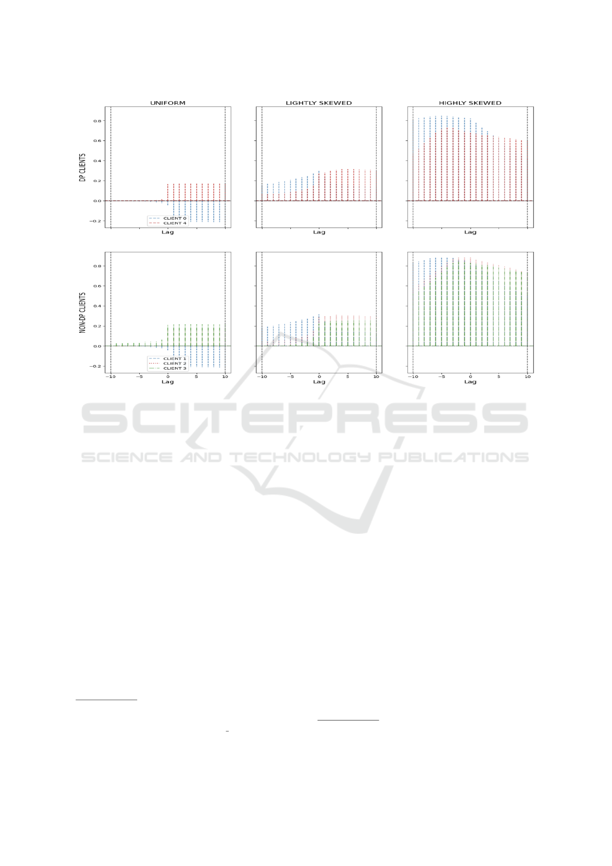
Figure 4: Cross-Correlation Function (CCF) plot for the CIFAR10 dataset for all three possible data splits. The y-axis contains

lag varying from -10 to +10 iterations, with lag equal to zero corresponding to the correlation between two variables. The

CCF for DP clients is placed in the ﬁrst row, and the corresponding values for non-DP clients are placed in the second row.

naling that the informativeness of the Shapley Values

in this context highly depends on the heterogeneity of

the system.

Given the experimental results, we clearly fail to

reject h

. The threshold is not met for 95% of the

test cases, with large p-values being evidenced across

all three types of data splits in the case of selected

datasets. However, some mildly informative patterns

could be observed, and we suggest how those patterns

could be utilized in the subsequent studies in the Con-

clusions of this work.

Regarding the formal hypothesis formulation, we

conclude that for the Spearman Correlation Test, we

fail to reject the null hypothesis h

, i.e.,, there is

no monotonic relationship between the two variables.

Similarly, we fail to reject h

for the linear relation-

ship between the variables using the Pearson Correla-

tion Test.

All tables in the tex format can be found

in the repository hosted for this submission:

https://github.com/Shapley-Mia/Shapley MIA/tree/main/

tables/correlations/pearson

5.3.4 Cross Correlation Test

The ﬁnal test performed for an assessment of the

be- haviour between those two variables is the vi-

sual in- spection of the Cross Correlation Function

(CCF). This test should allow us to answer the ques-

tion of whether there exists some meaningful relation-

ship between those two time series, where one series

is shifted in time by a lag τ.

Despite the lack of stationarity, absence of visi-

ble correlation, and failure to reject both hypotheses,

cross-correlation analysis provides an additional em-

pirical check. This ensures that a dishonest orches-

trator cannot extract meaningful information directly

from Shapley Values. The Cross Correlation Function

(CCF) - similar to the correlation analysis - shows

no clear patterns when it comes to how the Shapley

Value (SV) could possibly be used to detect the most

susceptible clients. We employ lags in the range of

values (−10, 10) to assess both the negative and posi-

tive lags. Figure 4 presents the value of correlation as-

sessed with lag τ ranging from −10 to 10 on a CIFAR-

10 dataset. Similar patterns are noticeable on other

datasets reported in our GitHub repository.

The rest of the available ﬁgures can be found in the

pre-generated notebook within the hosted repository: https:

SECRYPT 2025 - 22nd International Conference on Security and Cryptography

284

Figure 4 shows the cross-correlation function

(CCF) plot for each dataset across different data

splits. The ﬁrst row represents clients without a DP

mechanism, and the second row represents clients

with DP.

6 CONCLUSION

This work examined the relationship between client

contribution metrics, speciﬁcally Shapley Values, and

vulnerability to MIAs in a cross-silo FL setting. Our

results show that while Shapley Values offer insights

into client contributions, they do not inherently in-

crease the risk to MIA. Contrary to concerns, no con-

sistent correlation was found between Shapley Values

and the stages at which clients are most vulnerable to

MIAs.

We also report on a partial positive correlation that

sporadically emerged in our analysis with FashionM-

NIST and CIFAR-10. Here, higher SV were some-

times correlated with higher vulnerability to MIA

TPR. There is no statistical signiﬁcance here, but it

happened particularly for data splits of lesser hetero-

geneity. This suggests situations where clients are

characterised by similar local distributions, while the

orchestrator possesses an informative test set that ac-

curately reﬂects those distributions. One would like

to investigate further and propose hypotheses to test

because of these observations.

Future work will investigate whether the correla-

tion can appear under speciﬁc levels of data hetero-

geneity. We also aim to extend the analysis to other

privacy attacks, such as white-box MIAs, property in-

ference, and gradient leakage attacks, and to study the

effects of extreme data skew (e.g., Dirichlet α = 0.1).

Finally, formal proofs will be sought to validate the

underlying intuition linking Shapley Values and MIA

vulnerability.

ACKNOWLEDGEMENTS

This work was supported by EU projects LeADS

(GA no. 956562). Zuziak and Rinzivillo have

also been supported by the EU project TANGO (no.

101120763), while El Mestari and Lenzini by the EU

project NGSOTI (no. 101127921)

//github.com/MKZuziak/SECRYPT 2025 MIA SHAP/

blob/main/visualizations.ipynb

REFERENCES

Abadi, M., Chu, A., Goodfellow, I., and et al. (2016). Deep

learning with differential privacy. In Proceedings of

the 2016 ACM SIGSAC conference on computer and

communications security, pages 308–318.

Cohen, G., Afshar, S., Tapson, J., and et al. (2017). Em-

nist: Extending mnist to handwritten letters. In

2017 international joint conference on neural net-

works (IJCNN), pages 2921–2926. IEEE.

Dickey, D. A. and Fuller, W. A. (1979). Distribution of

the Estimators for Autoregressive Time Series With a

Unit Root. Journal of the American Statistical Asso-

ciation, 74(366):427–431. Publisher: [American Sta-

tistical Association, Taylor & Francis, Ltd.].

El Mestari, S. Z., Lenzini, G., and Demirci, H. (2024).

Preserving data privacy in machine learning systems.

Computers & Security, 137:103605.

Ghorbani, A. and Zou, J. (2019). Data Shapley: Eq-

uitable Valuation of Data for Machine Learning.

arXiv:1904.02868 [cs, stat].

Granger, C. W. J. (1969). Investigating Causal Relations

by Econometric Models and Cross-spectral Methods.

Econometrica, 37(3):424–438. Publisher: [Wiley,

Econometric Society].

Gu, Y., Bai, Y., and Xu, S. (2022). Cs-mia: Membership

inference attack based on prediction conﬁdence series

in federated learning. Journal of Information Security

and Applications, 67:103201.

Guo, W., Wang, Y., and Jiang, P. (2023). Incentive mech-

anism design for federated learning with stackelberg

game perspective in the industrial scenario. Comput.

Ind. Eng., 184(C).

Hestness, J., Narang, S., and et al. (2017). Deep learn-

ing scaling is predictable, empirically. arXiv preprint

arXiv:1712.00409.

Jain, A., Patel, H., and et al. (2020). Overview and impor-

tance of data quality for machine learning tasks. In

Proceedings of the 26th ACM SIGKDD international

conference on knowledge discovery & data mining,

pages 3561–3562.

Jia, R., Dao, D., and et al. (2019). Towards Efﬁcient Data

Valuation Based on the Shapley Value. In Proceedings

of the Twenty-Second International Conference on Ar-

tiﬁcial Intelligence and Statistics, pages 1167–1176.

PMLR. ISSN: 2640-3498.

Kairouz, P., McMahan, H. B., and et al. (2021). Ad-

vances and Open Problems in Federated Learning.

arXiv:1912.04977 [cs, stat]. arXiv: 1912.04977.

Koh, P. W. and Liang, P. (2017). Understanding black-box

predictions via inﬂuence functions. In International

conference on machine learning, pages 1885–1894.

PMLR.

Le, Y. and Yang, X. (2015). Tiny imagenet visual recogni-

tion challenge. CS 231N, 7(7):3.

Li, H., Meng, D., and et al. (2020a). Knowledge federa-

tion: A uniﬁed and hierarchical privacy-preserving ai

framework. In 2020 IEEE International Conference

on Knowledge Graph (ICKG), pages 84–91. IEEE.

Can Contributing More Put You at a Higher Leakage Risk? The Relationship Between Shapley Value and Training Data Leakage Risks in

Federated Learning

285

Li, Z., Lin, T., Shang, X., and Wu, C. (2023). Revisit-

ing Weighted Aggregation in Federated Learning with

Neural Networks. arXiv:2302.10911 [cs].

Li, Z., Sharma, V., and P. Mohanty, S. (2020b). Preserv-

ing Data Privacy via Federated Learning: Challenges

and Solutions. IEEE Consumer Electronics Magazine,

9(3):8–16. Conference Name: IEEE Consumer Elec-

tronics Magazine.

Liu, Z., Chen, Y., and et al. (2021). GTG-Shapley: Efﬁcient

and Accurate Participant Contribution Evaluation in

Federated Learning. arXiv:2109.02053 [cs].

Long, Y., Bindschaedler, V., and et al. (2018). Understand-

ing membership inferences on well-generalized learn-

ing models. arXiv preprint arXiv:1802.04889.

McMahan, H. and Moore, E. a. e. (2017). Communication-

efﬁcient learning of deep networks from decentralized

data. In Artiﬁcial intelligence and statistics, pages

1273–1282. PMLR.

Melis, L., Song, C., and et al. (2018). Infer-

ence attacks against collaborative learning. CoRR,

abs/1805.04049.

Nasr, M., Shokri, R., and Houmansadr, A. (2019). Compre-

hensive privacy analysis of deep learning: Passive and

active white-box inference attacks against centralized

and federated learning. In 2019 IEEE Symposium on

Security and Privacy (SP), pages 739–753.

Pearson, K. (1895). Note on Regression and Inheritance in

the Case of Two Parents. Proceedings of the Royal

Society of London, 58:240–242. Publisher: The Royal

Society.

Shapley, L. S. (1952). A Value for N-Person Games. Tech-

nical report, RAND Corporation.

Shokri, R., Stronati, M., and et al. (2017). Membership

inference attacks against machine learning models. In

2017 IEEE symposium on security and privacy (SP),

pages 3–18. IEEE.

Song, M., Wang, Z., Zhang, Z., and et al. (2020). Analyz-

ing user-level privacy attack against federated learn-

ing. IEEE Journal on Selected Areas in Communica-

tions, 38(10):2430–2444.

Song, T., Tong, Y., and Wei, S. (2019). Proﬁt Allocation for

Federated Learning. In 2019 IEEE International Con-

ference on Big Data (Big Data), pages 2577–2586.

Spearman, C. (1904). The Proof and Measurement of Asso-

ciation between Two Things. The American Journal

of Psychology, 15(1):72–101. Publisher: University

of Illinois Press.

Thakkar, O. D., Ramaswamy, S., and et al. (2021). Under-

standing unintended memorization in language mod-

els under federated learning. In Proceedings of the

Third Workshop on Privacy in Natural Language Pro-

cessing, pages 1–10, Online. Association for Compu-

tational Linguistics.

Wang, G., Dang, C. X., and Zhou, Z. (2019a). Measure

contribution of participants in federated learning. In

2019 IEEE international conference on big data (Big

Data), pages 2597–2604. IEEE.

Wang, G., Dang, C. X., and Zhou, Z. (2019b). Measure

Contribution of Participants in Federated Learning.

arXiv:1909.08525 [cs, stat].

Wang, J., Charles, Z., and et al. (2021). A Field Guide

to Federated Optimization. arXiv:2107.06917 [cs].

arXiv: 2107.06917.

Wang, T., Rausch, J., and et al. (2020). A Principled Ap-

proach to Data Valuation for Federated Learning. In

Yang, Q., Fan, L., and Yu, H., editors, Federated

Learning: Privacy and Incentive, Lecture Notes in

Computer Science, pages 153–167. Springer Interna-

tional Publishing, Cham.

Wei, S., Tong, Y., and et al. (2020). Efﬁcient and Fair Data

Valuation for Horizontal Federated Learning. In Yang,

Q., Fan, L., and Yu, H., editors, Federated Learn-

ing: Privacy and Incentive, Lecture Notes in Com-

puter Science, pages 139–152. Springer International

Publishing, Cham.

Yang, Q., Liu, Y., Chen, T., and Tong, Y. (2019). Federated

machine learning: Concept and applications. ACM

Transactions on Intelligent Systems and Technology

(TIST), 10(2):1–19.

Yousefpour, A., Shilov, I., and et al. (2021). Opacus: User-

friendly differential privacy library in pytorch. arXiv

preprint arXiv:2109.12298.

Zhang, J., Zhang, J., and et al. (2020). Gan enhanced mem-

bership inference: A passive local attack in federated

learning. In ICC 2020 - 2020 IEEE International Con-

ference on Communications (ICC), pages 1–6.

Zheng, S., Cao, Y., and Yoshikawa, M. (2023). Se-

cure Shapley Value for Cross-Silo Federated Learn-

ing. arXiv:2209.04856 [cs].

SECRYPT 2025 - 22nd International Conference on Security and Cryptography

286