Design and Application of the BMFCP Architecture in Flight Simulation

Systems

Jiaxuan Zhang

, Runkai Ji and Guanxin Hong

School of Aeronautic Science and Engineering, Beihang University, Beijing, China

Keywords:

Flight Simulation, Flight Dynamic, OOP, Software Architecture Design.

Abstract:

Flight simulation plays a crucial role in aircraft conceptual design, guidance and control system development,

and pilot training. To address the limitations in the architectural design of the dynamics core in traditional ﬂight

simulation systems, this study proposes a novel architecture: Boundary-Motion-Force-Coordinate-Parameter

(BMFCP), based on the characteristics of ﬂight dynamics problems and object-oriented software development

techniques. The BMFCP architecture decomposes the dynamics core of ﬂight simulation systems into three

layers: the boundary layer, the motion equation layer, and the external force layer, along with two packages:

the coordinate transformation package and the parameter package. Using a ﬂight simulation system based

on the BMFCP architecture, simulations of carrier-based aircraft landing and seaplane takeoff and landing

processes were successfully conducted. Thanks to the design of this architecture, different ﬂight simulation

tasks can be achieved by simply modifying the code in the external force layer to simulate various aircraft.

Analysis of the simulation results shows that the time-domain curves of aircraft position and attitude align

with empirical observations, validating the correctness of the ﬂight simulation system based on the BMFCP

architecture.

1 INTRODUCTION

The ﬂight process is inherently risky and uncertain,

especially for newly designed aircraft and inexpe-

rienced pilots. Conducting ﬂight missions without

comprehensive aircraft performance evaluation and

pilot training signiﬁcantly increases the probability of

aircraft accidents. Flight simulation, which uses com-

puters or other devices to simulate aircraft motion and

control in real-world environments, plays a crucial

role in aircraft design and pilot training. In the ﬁeld

of aircraft design and controller development, (Zhang

et al., 2024) highlights that conducting ﬂight simu-

lations during the structural design phase can evalu-

ate the operational performance of the aircraft. Simi-

larly, (Zhao et al., 2024) emphasizes that software-in-

the-loop (SITL) simulations can validate control al-

gorithms for aircraft. Regarding pilot training, (Caro,

1973) suggests that training time on ﬂight simulators

can replace actual ﬂight training time, while (Thom-

son, 1989) points out that the degree to which simu-

lators can replace real ﬂight training depends on their

ﬁdelity. (Allerton, 2009) notes that compared to the

1970s, when real ﬂights were used for training, mod-

https://orcid.org/0009-0008-2753-4885

ern simulator-based training has signiﬁcantly reduced

the number of training-related accidents. Addition-

ally, (Maciejewska et al., 2024) highlights the eco-

nomic advantages of simulator-based training.

In recent years, ﬂight simulation technology has

shown a rapid development trend. Firstly, the ﬁdelity

of models has always been a key focus of related re-

search. (Milne et al., 2023) achieved accurate calcu-

lations of aeroelasticity, turbulence, atmosphere, and

other effects during high-ﬁdelity motion simulations

of sounding rockets, laying the foundation for virtual

sensing and digital twins in autonomous navigation

and guidance. (An et al., 2022) utilized the ﬂight

dynamic model, helicopter trim, linearization, and

simulation (HETLAS) system for high-ﬁdelity mo-

tion simulations of complex-conﬁgured aircraft, ef-

fectively describing traditional helicopters, propeller-

driven ﬁxed-wing aircraft, and more complex air-

craft conﬁgurations. (Rezaei and Khosravi, 2022) im-

proved the ﬁdelity of actuator models by conducting

parametric model identiﬁcation using aircraft system

data. Secondly, (Dhiman et al., 2025) pointed out

that artiﬁcial intelligence and data-driven technolo-

gies are gradually being applied to aircraft model-

ing and simulation. (Cao et al., 2022) proposed an

374

Zhang, J., Ji, R. and Hong, G.

Design and Application of the BMFCP Architecture in Flight Simulation Systems.

DOI: 10.5220/0013637000003970

In Proceedings of the 15th International Conference on Simulation and Modeling Methodologies, Technologies and Applications (SIMULTECH 2025), pages 374-381

ISBN: 978-989-758-759-7; ISSN: 2184-2841

interpretable learning algorithm for aircraft systems,

adaptive-SINDYc, to identify aircraft models. (Pun-

jani and Abbeel, 2015) employed a rectiﬁed linear

unit (ReLU) network model to represent helicopter

dynamics.

Although recent advancements in ﬂight simula-

tion technology have been signiﬁcant, limited atten-

tion has been paid to the architectural design of the

dynamics core in ﬂight simulation systems. A well-

designed dynamics core architecture can offer relia-

bility, reusability, readability, maintainability, and ex-

pandability advantages. An effective architecture of a

dynamics core must integrate various object-oriented

techniques in software design and key algorithms for

ﬂight dynamics problems. To this end, this study an-

alyzes the establishment of aircraft motion models,

key algorithms in ﬂight simulation, and the architec-

tural design of the dynamics core. A novel archi-

tecture termed Boundary-Motion-Force-Coordinate-

Parameter (BMFCP) is proposed. Using a ﬂight simu-

lation system based on the BMFCP architecture, sim-

ulations of carrier-based aircraft landing and seaplane

takeoff and landing processes were successfully con-

ducted. The simulation results validate the correct-

ness and effectiveness of the ﬂight simulation system

based on BMFCP architecture.

2 FLIGHT MOTION MODEL IN

WIND FIELDS

The aircraft motion model in wind ﬁelds serves as

the core model driving the ﬂight simulation system.

This section establishes both the full nonlinear mo-

tion model suitable for unsteady operating conditions

and the linearized motion model suitable for steady

operating conditions.

2.1 Deﬁnition of Coordinate Systems

and Motion Parameters

We adopt the local tangent plane coordinate system

LTP

as the ﬁxed coordinate system, with the x-axis

pointing north, the y-axis pointing east, and the origin

located at the mean sea level. A ﬂight body coordi-

nate system S

f b

is established to describe the absolute

position and attitude of the aircraft. The origin of S

f b

is located at the aircraft’s center of mass CM, with

the x-axis pointing forward, the y-axis pointing to the

right, and the z-axis determined by the right-hand rule

pointing downward. The absolute motion parameters

of the aircraft can be determined by the relative posi-

tion relationship between S

f b

and S

LTP

. Speciﬁcally,

the absolute position r

of the aircraft is deﬁned as

the vector from point O

LTP

to point CM as follows.

= r

CM←O

LTP

(1)

The aircraft’s attitude Euler angles, including

pitch angle φ

, roll angle θ

, and yaw angle ψ

, are

deﬁned as a set of Euler angles that transform the S

LTP

to the S

f b

using a z − y − x rotation sequence. the ab-

solute Euler angle vector of the aircraft Θ

∈ R

deﬁned as follows.





⊤

(2)

The aerodynamic coordinate system S

describes

the incoming airﬂow relative to the aircraft. The ori-

gin of this coordinate system is located at the aircraft’s

aerodynamic center (AC). The x-axis is aligned with

the direction of the airﬂow velocity vector v

, point-

ing towards the aircraft’s nose. The z-axis lies within

the aircraft’s symmetry plane, perpendicular to v

and points downward. The y-axis is determined by

the right-hand rule, pointing to the right side of the

aircraft.

The aerodynamic angles of the aircraft, including

the angle of attack α

and the sideslip angle β

, can be

deﬁned through the transformation relationship from

f b

to S

as follows

f b

(−α

)

−−−−−−−→ ◦

(β

)

−−−−−−−→ S

(3)

based on the above relationship, the angle of attack α

and the sideslip angle β

of the aircraft can be derived

from the components of the airﬂow velocity vector v

in S

f b

as follows.

= arctan



a,z f b

a,x f b



= arcsin



a,y f b













(4)

The ﬂight path coordinate system S

is used to de-

scribe the aircraft’s ﬂight path and track velocity v

The origin of this coordinate system is located at the

aircraft’s center of mass CM. The x-axis is aligned

with the track velocity v

and points towards the air-

craft’s nose. The z-axis is perpendicular to the x-axis

and lies in a vertical plane, pointing downward. The

y-axis is determined by the right-hand rule and points

to the right side of the aircraft.

The ﬂight path angles, including the track azimuth

angle χ

and the track inclination angle γ

, can be

deﬁned through the transformation relationship from

LTP

to S

as follows

LTP

(χ

)

−−−−−−−→ ◦

(γ

)

−−−−−−−→ S

(5)

Design and Application of the BMFCP Architecture in Flight Simulation Systems

375

based on the above relationship, the track azimuth an-

gle χ

and the track inclination angle γ

of the aircraft

can be derived from the components of the track ve-

locity vector v

in S

LTP

as follows.

= arcsin



−

k, zLT P



= arctan



k, yLT P

k, xLT P













(6)

2.2 Full Nonlinear Motion Model

For a rigid body undergoing general motion, based

on the general motion equations of a rigid body with

respect to its center of mass, the equations of motion

for an aircraft in Euler angle form are expressed as

follows











f b





f b



dω



f b













)

f b

−1

(ω

)

f b

−1

)

f b

)

−1

f b

f ↢O

)

f b

− (ω

)

f b

)

f b

(ω

)

f b







(7)

where F

represents the resultant external force act-

ing on the aircraft; M

f ↢O

denotes the resultant ex-

ternal moment about the center of mass; (J

)

f b

is the

inertia matrix of the aircraft relative to its center of

mass and S

f b

; D

is the transformation matrix from

Euler angle rates to angular velocity.

The resultant external force F

and moment

f ↢O

acting on most aircraft consist of three com-

ponents: aerodynamic force, gravitational force, and

thrust. The aerodynamic force F

f a

and moment

f a↢O

can be expressed as follows

f a

)

f b

= ¯qSR

⊤

a← f b



−C



⊤

(8)

f a↢O

)

f b

= ¯qSR

⊤

a← f b



¯cC



⊤

+ (r

AC←CM

)

f b

× (F

f a

)

f b

(9)

where C

represent the drag coef-

ﬁcient, side force coefﬁcient, lift coefﬁcient, rolling

moment coefﬁcient, pitching moment coefﬁcient, and

yawing moment coefﬁcient, respectively. These pa-

rameters are functions of the aircraft’s motion and

aerodynamic parameters, typically obtained through

wind tunnel experiments or computational ﬂuid dy-

namics (CFD) methods. In simulations, these param-

eters are often retrieved via lookup tables. S denotes

the wing area, b the wingspan, ¯c the mean aerody-

namic chord, ¯q the dynamic pressure, and r

AC←CM

the

vector from the aircraft’s CM to AC.

The gravitational force F

f g

acting on the aircraft,

expressed in S

f b

is given as follows

f g

)

f b

= R

f b←LTP



0 0 −m



⊤

(10)

where m

represents the mass of the aircraft, and g

denotes the gravitational acceleration.

The thrust F

f t

generated by the aircraft engine and

the additional moment M

f t

induced by its installation

can be expressed as follows

f t

)

= R

⊤

(θ

eng,ins

)



T 0 0



⊤

(11)

f t

)

= (r

eng← f b

)

f b

× (F

f t

)

f b

(12)

where θ

eng,ins

represents the engine installation angle,

T denotes the engine thrust, and r

eng← f b

is the posi-

tion vector of the engine thrust center relative to the

aircraft’s center of mass.

The inputs to the aircraft dynamics system include

ﬁve control variables: the left and right elevator de-

ﬂections δ

,δ

, the aileron deﬂection δ

, the rudder

deﬂection δ

, and the throttle setting τ. Additionally,

there are three wind ﬁeld disturbances, represented

by the components of the wind velocity vector v

T LP

: u

w,LT P

The essence of full nonlinear ﬂight simulation lies

in the numerical integration of complex nonlinear dif-

ferential equations. In the simulation, the continuous

states are denoted as c

c, the discrete states as d

d, the

inputs as i

i, and the outputs as o

o, with time t being a

proper subset of the inputs t ⊂ i

i. The full nonlinear

ﬂight simulation can be expressed as the following set

of equations

c = f (c

c,d

d, i

d = g(c

c,i

o = h(c

c,d

d, i











(13)

where f (c

c,d

d, i

i) represents the continuous state equa-

tions, which, in the context of ﬂight simulation, cor-

respond to the equations of motion shown in Eq. 7.

However, certain aircraft state variables, such as the

angle of attack α

, are not part of c

c but directly

inﬂuence the computation on the right-hand side of

Eq. 7. These parameters can be derived using alge-

braic equations g(c

c,i

i) related to the continuous states

c and inputs i

i, such as Eq. 4. To provide comprehen-

sive simulation results, the outputs o

o are deﬁned as a

combination of the continuous states c

c, their deriva-

tives

c, and the discrete states d

2.3 Linearized Motion Model

When an aircraft performs steady-state motion (e.g.,

steady-level ﬂight or steady descent), its motion can

SIMULTECH 2025 - 15th International Conference on Simulation and Modeling Methodologies, Technologies and Applications

376

be well represented by a linearized model under small

perturbation conditions.

We deﬁne the state variables ∆X

X ∈ R

and input

variables ∆U

U ∈ R

for the aircraft as follows

∆X

X =





∆Θ

∆(v

)

f b

∆(ω

)

f b





(14)

∆U

U =







∆δ

∆τ

∆u

w,LT P

∆v

w,LT P

∆w

w,LT P







(15)

where ∆ represents the perturbation relative to the

trim state. In the linearized motion model, we select

the system output as ∆Y

Y = ∆X

X. Additional outputs,

such as the angle of attack α

and sideslip angle β

can be obtained through nonlinear calculations based

on the state variables ∆X

X and input variables ∆U

U. The

aircraft’s position can be determined by integrating

the velocity.

The linearized motion model of the aircraft can

be expressed in the form of the following state-space

equations

∆

X = A

A∆X

X +B

B∆U

∆Y

Y = ∆X

(16)

where A

A and B

B are the Jacobian matrices of the state-

space equations, deﬁned as follows

A =

∂

∂ X



trim

B =

∂

∂U



trim

(17)

where X

trim

and U

trim

represent the state variables

and input variables of the aircraft in the trimmed con-

dition, respectively.

3 BMFCP ARCHITECTURE

DESIGN IN FLIGHT

SIMULATION SYSTEMS

This study is based on key issues in ﬂight dynam-

ics and incorporates object-oriented software design

techniques to propose a Boundary-Motion-Force-

Coordinate-Parameter (BMFCP) architecture for the

dynamics core of ﬂight simulation systems. The BM-

FCP architecture is based on the Boundary-Control-

Entity (BCE) three-layer architecture proposed by

(Martin, 2002), with adaptive improvements tailored

to ﬂight dynamics problems. This architecture of-

fers advantages in reliability, reusability, readability,

maintainability, and extensibility.

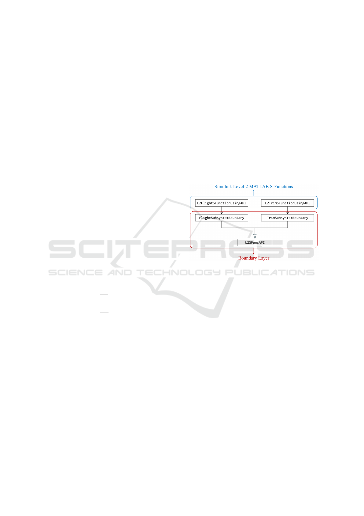
3.1 Boundary Layer Design

In the BMFCP architecture, the Boundary Layer is re-

sponsible for interactions between the system and its

actor. The design of the Boundary Layer adheres to

the interface segregation principle (ISP) proposed by

(Martin, 1996). Taking interaction with the Simulink

system as an example, the class diagram of the bound-

ary layer interacting with Simulink is shown in Fig-

ure 1. Where the Simulink Level-2 MATLAB S-

Function is a tool in Simulink used for creating cus-

tom Simulink block interfaces using MATLAB code.

Figure 1: Class Diagram of the Boundary Layer.

3.2 Motion Equation Layer Design

The motion equation layer in the BMFCP architecture

corresponds to the control layer in the BCE three-

layer architecture. Since the motion equations are

applicable to any aircraft under any operating condi-

tions, this layer is the most stable and invariant in de-

sign. The class diagram of the motion equation layer

is shown in Figure 2. The CalcDerivatives class

is responsible for solving the continuous state deriva-

tives of the aircraft, corresponding to the function

˙c = f (c,d,i) in Eq. 13. The UpdateDiscStates class

is used to compute the discrete states of the aircraft,

corresponding to the function d = g(c,i) in Eq. 13.

The DynamicEquation class describes the aircraft’s

dynamic equations as shown in Eq. 7.

3.3 External Force Layer Design

The external force layer in the BMFCP architecture

corresponds to the Entity Layer in the BCE three-

layer architecture. Due to the varying force calcula-

tion methods for different aircraft, the design of the

Design and Application of the BMFCP Architecture in Flight Simulation Systems

377

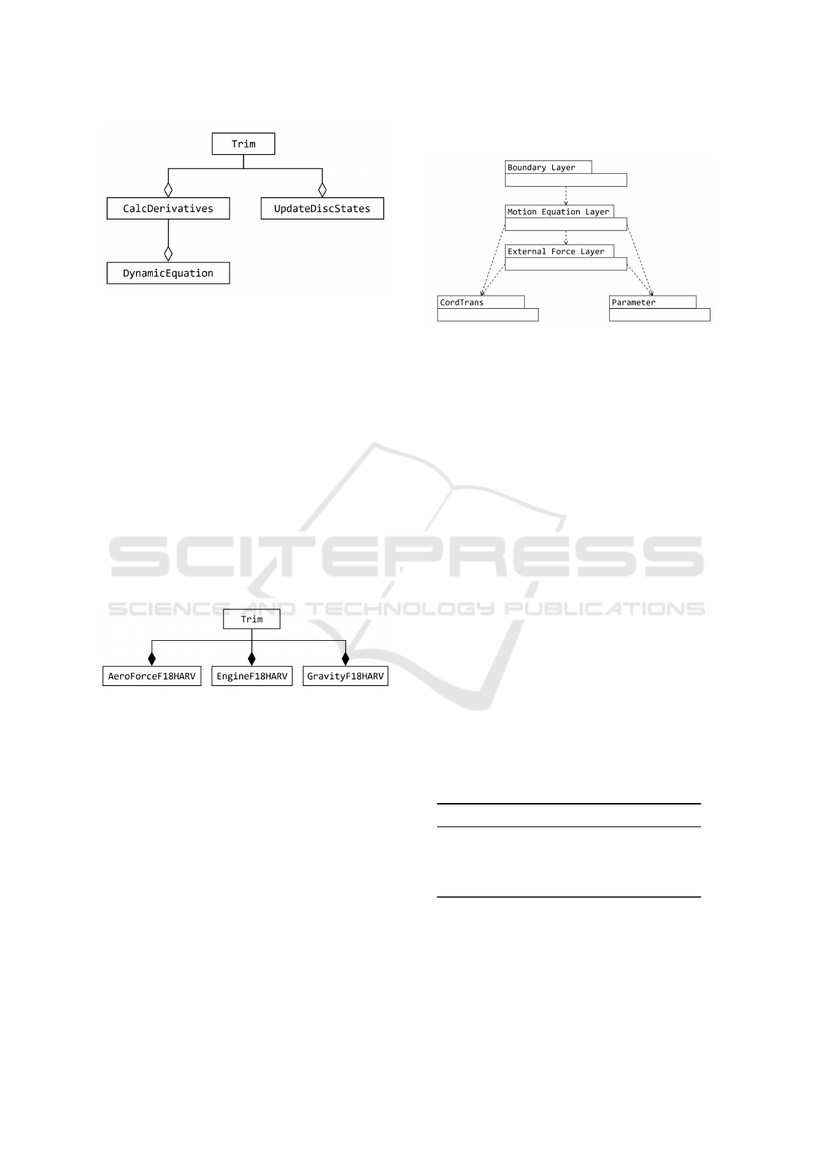
Figure 2: Class Diagram of the Motion Equation Layer.

external force layer must be interchangeable and ex-

tensible. For instance, when simulating the F-18 High

Angle of Attack Research Vehicle (HARV), the class

diagram of the external force layer is shown in Fig-

ure 3. The resultant force class, ResultantForce,

comprises several sub-forces. According to the

Liskov substitution principle proposed by (Liskov

and Wing, 1994), the classes AeroForceF18HARV,

EngineF18HARV, and GravityF18HARV in the exter-

nal force layer can be replaced with classes describing

the forces acting on other aircraft, thereby enabling

simulations for different aircraft. Following the open-

closed principle (OCP) proposed by (Meyer, 1988),

the sub-force classes in the external force layer can be

extended. For example, additional classes describing

hydrodynamic forces and buoyancy can be added to

simulate seaplanes, thereby expanding the simulation

capabilities for such aircraft.

Figure 3: Class Diagram of the External Force Layer.

3.4 BMFCP Architecture Design

In addition to the three primary layers men-

tioned earlier, the BMFCP architecture also in-

cludes two packages: the coordinate transforma-

tion package (CordTrans) and the parameter pack-

age (Parameter). The CordTrans package provides

frequently used coordinate transformation methods,

while the Parameter package allows for the deﬁni-

tion of constants in the MATLAB environment, offer-

ing the advantage of easily switching between differ-

ent aircraft parameters. Since these two packages are

respectively dependent on the motion equation layer

and the external force layer, the overall package dia-

gram of the BMFCP architecture is proposed in accor-

dance with the acyclic dependencies principle (ADP)

introduced by (Martin, 2002), as shown in Figure 4.

Figure 4: Architecture Package Diagram.

4 SIMULATION RESULT

To facilitate the design of carrier-based aircraft land-

ing guidance and control laws, as well as the con-

ceptual design of seaplanes, we conducted simulation

studies on the landing process of a carrier-based air-

craft and the takeoff and landing processes of a sea-

plane. In this section, we present the results of these

simulations and analyze their outcomes.

4.1 Case Study of Carrier-Based

Aircraft Landing

Due to the track inclination angle γ

is a constant dur-

ing carrier-based aircraft landing, operating condition

above is a steady-state condition. Therefore, using a

linearized aircraft model for simulation is appropriate.

In this study, the F-18 HARV is used as the test air-

craft, with its parameters sourced from (Asbury and

Capone, 1995), (Iliff, 1997), and (Iliff, 1999). The

aircraft is trimmed to a position where its tailhook is

50 meters below the commanded altitude to evaluate

the performance of the guidance and control system.

The speciﬁc trim parameters are shown in Table 1.

Table 1: Carrier-Based Flight Landing Trim Parameter.

Parameter Trim value

Initial hook height error, h

he0

[m] -50

Track inclination angle, γ

[Deg] -4

Track speed, V

[m/s] 80

Pitch angle, θ

[Deg] 2.15

The aircraft’s tailhook’s absolute and commanded

heights are shown as the blue and red lines in Figure 5,

respectively. The simulation results indicate that the

aircraft corrects the tailhook height error within ap-

proximately 20 seconds and effectively maintains the

SIMULTECH 2025 - 15th International Conference on Simulation and Modeling Methodologies, Technologies and Applications

378

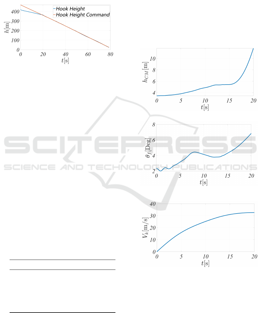
commanded tailhook height during the ﬁnal approach

phase before touchdown. These results demonstrate

the effectiveness of the ﬂight simulation system based

on the BMFCP architecture when conducting simula-

tions using linearized models.

Figure 5: Carrier-Based Flight Landing Height.

4.2 Case Studies of Seaplane Takeoff

and Landing

Seaplanes are aircraft capable of taking off and

landing on water surfaces. Simulating the takeoff

and landing processes during the preliminary design

phase can facilitate rapid iterative optimization of de-

sign schemes. Due to seaplane takeoff and landing

operations’ highly complex, nonlinear, and unsteady

nature, the aircraft’s full nonlinear motion model must

be employed for simulation. Thanks to the design

of the external force layer in the BMFCP architec-

ture, seaplane takeoff and landing simulation can be

achieved by simply adding classes that describe hy-

drodynamic forces and buoyancy to this layer.

This study conducted a simulation of the takeoff

process for a speciﬁc type of seaplane. The seaplane’s

takeoff process includes three stages: stationary ﬂoat-

ing on the water, water taxiing, and liftoff. The sim-

ulation begins with the aircraft ﬂoating stationary on

the water, with the control surfaces trimmed to a state

corresponding to a ﬁxed track inclination angle γ

during ascent. Table 2 shows the speciﬁc trim param-

eters.

Table 2: Seaplane Takeoff Trim Parameter.

Parameter Trim value

CM height, h

[m] 3.34

Pitch angle, θ

[Deg] 2.34

Elevator angle, δ

[Deg] -5.92

Aileron angle δ

[Deg] 0

Rudder angle δ

[Deg] 0

Throttle 1

The time-domain simulation results of the sea-

plane takeoff process are shown in Figure 6. The re-

sults indicate that the aircraft lifts off from the wa-

ter surface approximately 15 seconds after starting

from rest. After liftoff, the aircraft continues to climb,

reaching an altitude of h

= 10m with a track incli-

nation angle of γ

≈ 0.5

◦

. The track velocity V

sta-

bilizes around 30m/s after liftoff. These results are

consistent with the actual takeoff process of a sea-

plane, validating the effectiveness of the ﬂight simu-

lation system based on the BMFCP architecture when

conducting simulations using the full nonlinear mo-

tion model.

(a) Takeoff CM height.

(b) Takeoff Pitch angle.

Figure 6: Time Domain Curve of Seaplane Takeoff.

This study also conducted a simulation of the

landing process for a speciﬁc type of seaplane. The

landing process of the seaplane includes three stages:

steady descent, water touchdown, and deceleration

during water taxiing. The simulation begins with the

Design and Application of the BMFCP Architecture in Flight Simulation Systems

379

aircraft in a steady descent state, with the control

surfaces and attitude trimmed to maintain a steady

descent condition. The speciﬁc trim parameters are

shown in Table 3.

Table 3: Seaplane Landing Trim Parameter.

Parameter Trim value

CM height, h

[m] 10

Track inclination angle, γ

[Deg] -0.5

Track speed, V

[m/s] 30.3

Pitch angle, θ

[Deg] 4.03

Angle of attack, α

[Deg] 4.53

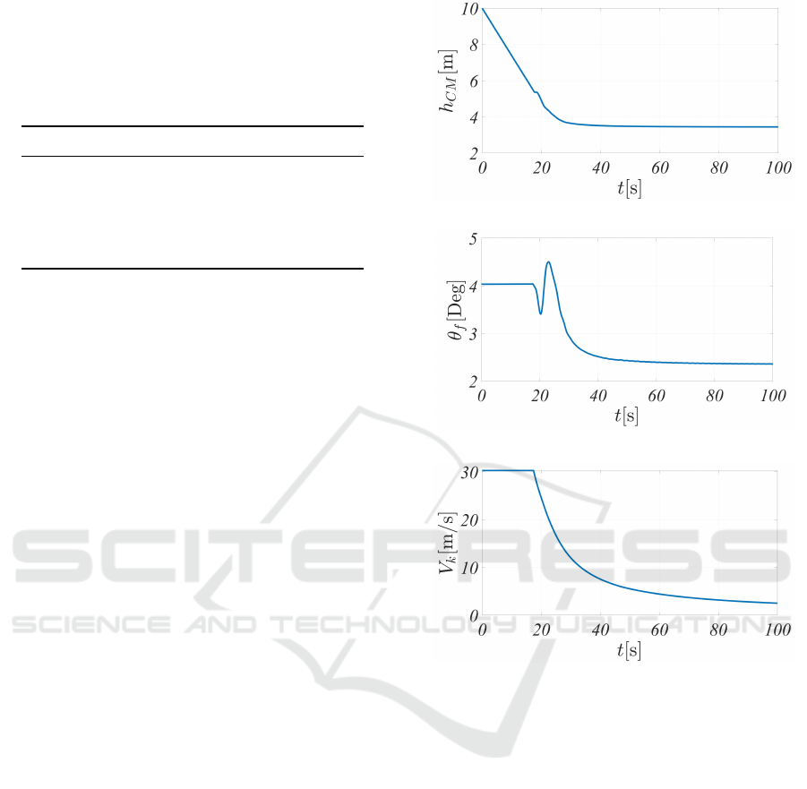
The time-domain simulation results of the sea-

plane landing process are shown in Figure 7. The sim-

ulation results indicate that the aircraft touches down

on the water surface at approximately 17 seconds. Af-

ter touchdown, the track velocity V

decreases rapidly

and reduces to approximately 2.5m/s at 100 seconds.

The pitch angle θ

and angle of attack α

exhibit ﬂuc-

tuations of around 1

◦

upon water impact due to hy-

drodynamic forces. These results are consistent with

the actual landing process of a seaplane, validating

the effectiveness of the ﬂight simulation system based

on the BMFCP architecture when conducting simula-

tions using the full nonlinear motion model.

5 CONCLUSIONS

This study, through an in-depth analysis of ﬂight dy-

namics problems and their key algorithms, combined

with object-oriented software design techniques,

proposes a Boundary-Motion-Force-Coordinate-

Parameter (BMFCP) architecture applicable to the

dynamics core of ﬂight simulation systems. This

architecture enhances ﬂight simulation systems’

reliability, reusability, readability, maintainability,

and extensibility. These advantages signiﬁcantly

reduce modiﬁcation costs and failure probabilities

when conducting ﬂight simulations for different

aircraft and operation conditions.

This study presents and analyzes two sets of sim-

ulation results based on the linearized and full nonlin-

ear motion models of aircraft, focusing on the carrier-

based aircraft landing process and the seaplane take-

off and landing processes. The results validate the ef-

fectiveness of the ﬂight simulation system based on

the BMFCP architecture in conducting simulations

using both linearized and full nonlinear models. Fur-

thermore, the study highlights the signiﬁcant role of

this simulation system in the design of aircraft guid-

ance and control laws and overall aircraft design. Ad-

(a) Takeoff CM height.

(b) Takeoff Pitch angle.

Figure 7: Time Domain Curve of Seaplane Landing.

ditionally, the system demonstrates potential as the

dynamics core of ﬂight simulators, with promising fu-

ture pilot training applications.

REFERENCES

Allerton, D. (2009). Principles of Flight Simulation. Wiley.

An, J.-Y., Choi, Y.-S., Lee, I.-R., Lim, M., and Kim, C.-

J. (2022). Performance analysis of a conceptual ur-

ban air mobility conﬁguration using high-ﬁdelity ro-

torcraft ﬂight dynamic model. Int. J. Aeronaut. Space

Sci., 24:1491–1508.

Asbury, S. C. and Capone, F. J. (1995). Multiaxis thrust-

vectoring characteristics of amodel representative of

the f-18 high-alpharesearch vehicle at angles of attack

from 0°to 70°. Technical report, Langley Research

Center.

Cao, R., Lu, Y., and He, Z. (2022). System identiﬁcation

SIMULTECH 2025 - 15th International Conference on Simulation and Modeling Methodologies, Technologies and Applications

380

method based on interpretable machine learning for

unknown aircraft dynamics. Aerospace Science and

Technology, 126:107593.

Caro, P. W. (1973). Aircraft simulators and pilot training.

Human Factors, 15:502–509.

Dhiman, G., Tiumentsev, A. Y., and Tiumentsev, Y. V.

(2025). Neural network and hybrid methods in air-

craft modeling, identiﬁcation, and control problems.

Aerospace, 12(1).

Iliff, K. W. (1997). Flight-determined subsonic longitudi-

nalstability and control derivatives of the f-18high an-

gle of attack research vehicle (harv)with thrust vector-

ing. Technical report, Dryden Flight Research Center.

Iliff, K. W. (1999). Flight-determined, subsonic, lateral-

directional stability and control derivatives of the

thrust-vectoring f-18 high angle of attack research ve-

hicle (harv), and comparisons to the basic f-18 and

predicted derivatives. Technical report, Dryden Flight

Research Center.

Liskov, B. and Wing, J. (1994). A behavioral notion of

subtyping. ACM Transactions on Programming Lan-

guages and Systems (TOPLAS), 16(6):1811–1841.

Maciejewska, M., Kurzawska-Pietrowicz, P., Galant-

Gołe¸biewska, M., Gołe¸biewski, M., and Jasi

nski, R.

(2024). Ecological and cost advantage from the im-

plementation of ﬂight simulation training devices for

pilot training. Applied Sciences, 14(18).

Martin, R. C. (1996). The interface segregation principle.

C++ Report, 8(7):57–62.

Martin, R. C. (2002). Agile Software Development: Princi-

ples, Patterns, and Practices. Prentice Hall.

Meyer, B. (1988). Object-Oriented Software Construction.

Prentice Hall.

Milne, B., Samson, S., Carrese, R., Gardi, A., and Sabatini,

R. (2023). High-ﬁdelity dynamics modelling for the

design of a high-altitude supersonic sounding rocket.

Designs, 7(1).

Punjani, A. and Abbeel, P. (2015). Deep learning helicopter

dynamics models. In 2015 IEEE International Con-

ference on Robotics and Automation (ICRA), pages

3223–3230.

Rezaei, P. and Khosravi, A. (2022). Parametric model iden-

tiﬁcation of nonlinear aircraft system with actuator

saturation. In 2022 International Conference on Smart

Information Systems and Technologies (SIST), pages

1–4.

Thomson, D. R. (1989). Transfer of training from simula-

tors to operational equipment—are simulators effec-

tive? Journal of Educational Technology Systems,

17(3):213–218.

Zhang, S., Tong, C., Ni, Y., Li, N., and Lin, Z. (2024).

Structural design and ﬂight simulation of ﬁreﬁghting

and rescue uav based on coaxial dual rotors. Inter-

national Journal of Pattern Recognition and Artiﬁcial

Intelligence, 38(12):2458004.

Zhao, W., Wang, Y., Li, L., Huang, F., Zhan, H., Fu, Y., and

Song, Y. (2024). Design and ﬂight simulation veriﬁ-

cation of the dragonﬂy evtol aircraft. Drones, 8(7).

Design and Application of the BMFCP Architecture in Flight Simulation Systems

381