Weather Forecasting Using Multilayer Perceptron Technique

Shifanaaz Abdulsab Nadaf

, Afrasama A. Harlapur

, Fathma Shekh

, Aleena A. Sayed

and Shashank Hegde

School of Computer Science and Engineering, KLE Technological University, Vidyanagar, Hubballi, India

Keywords:

Cosine Annealing Scheduler, Hyperparameter Tuning, Multi-Layer Perceptron (MLP), Weather Forecasting,

Neural Network Depth.

Abstract:

The Multilayer Perceptron (MLP) in weather forecasting is used for regression tasks based on input features

such as pressure values, temperature, pressure values, wind. This proposed work focuses on evaluating the

efﬁciency of MLP for accurate time series pattern predictions. This study incorporates ERA5 hourly data on

pressure levels from 1940 to the present and uses a Feedforward Neural Network(FNN) MLP architecture. In

addition, techniques such as the Cosine Annealing Learning Rate Scheduler and Hyperparameter Tuning are

employed to analyze temporal relationships, perform feature selection and ultimately improve model perfor-

mance. Experiments conducted with MLPs demonstrate competitive accuracy with MSE 91.92, MAE 7.02

and R² 0.9985 compared to traditional forecasting models, highlighting MLPs as a valid method for meteoro-

logical applications.

1 INTRODUCTION

Weather forecasting plays a crucial role in under-

standing the dynamics of the atmosphere and is

critical for numerous industries, including agricul-

ture, transportation, energy, and disaster manage-

ment.(Jaseena and Kovoor, 2022) The process of

predicting the weather condition for the future is

known as weather forecasting.(Singh et al., 2019) It

reduces risks, maximizes agricultural yields, allows

safe transportation, and enables proper energy man-

agement. The use of real-time temperature, humid-

ity, and pressure data using various sensors(Singh

et al., 2019). The task of weather forecasting is in-

herently challenging because atmospheric systems are

complex and unpredictable and Artiﬁcial Neural Net-

works (ANNs) have some interesting properties that

made this family of machine learning algorithms very

appealing when confronted with difﬁcult pattern dis-

covery tasks.(Fente and Singh, 2018)

Traditional models of weather forecasting usually

fail to account for many inherent nonlinearities and

complexities in the data. They tend to focus more

on the broad strokes among the fundamental atmo-

https://orcid.org/0009-0002-6067-6136

https://orcid.org/0009-0000-7179-1389

https://orcid.org/0009-0001-0556-883X

https://orcid.org/0009-0007-0421-9279

spheric variables that comprise temperature, pressure,

moisture, and wind. As a result, they often produce

less reliable forecasts of the weather, especially in the

long range or for regions where the weather changes

rapidly.

Pressure is one of the primary atmospheric vari-

ables and, thus, holds meteorological importance

as its changes mark weather fronts, high- or low-

pressure systems, etc. Therefore, accurate predictions

of pressure levels are likely to provide essential in-

formation regarding the atmospheric pattern at var-

ious altitudes, and in general, it enhances the over-

all accuracy of weather prediction. However, even

in the present day models, pressure levels cannot be

predicted accurately, which leads to a call for more

advanced techniques.

This paper explores the possibility of using Mul-

tilayer Perceptrons, a form of artiﬁcial neural net-

work, to overcome these challenges. MLPs have been

shown to be capable of capturing complex, nonlin-

ear relationships between atmospheric variables. Un-

like traditional forecasting methods, MLPs can pro-

cess large historical datasets and uncover subtle pat-

terns and correlations that conventional approaches

might overlook. This makes MLPs a powerful tool

for improving the accuracy and reliability of weather

forecasts.

The purpose of this research is to use MLPs to

360

Nadaf, S. A., Harlapur, A. A., Shekh, F., Sayed, A. A. and Hegde, S.

Weather Forecasting Using Multilayer Perceptron Technique.

DOI: 10.5220/0013616600004664

Paper published under CC license (CC BY-NC-ND 4.0)

In Proceedings of the 3rd International Conference on Futuristic Technology (INCOFT 2025) - Volume 3, pages 360-367

ISBN: 978-989-758-763-4

develop an efﬁcient and accurate forecasting model

for atmospheric pressure levels. There are two types

of data mining tasks: descriptive data mining tasks

that describe the general properties of existing data

and predictive data mining tasks that attempt to

make predictions based on inference from available

data.(Bushara and Abraham, 2014) This proposed

model will use high-resolution historical data from

sources such as the ERA5 dataset(Zhong et al., 2024)

to model the intricate interactions between various at-

mospheric variables while ensuring high accuracy in

predictions.

The primary objectives of this proposed model are

to develop and train an MLP model for weather fore-

casting, especially focusing on the prediction of pres-

sure levels. The model will be designed to capture the

complex interactions among atmospheric variables

and, therefore, provide a more accurate representation

of pressure variations. It generates the data set assim-

ilating high-quality and abundant global observations

with ECMWF’s IFS model(Chen et al., 2023).

The performance of the developed MLP model

shall be evaluated with Established performance met-

rics also used include Mean Absolute Error (MAE),

Mean Squared Error (MSE), and R-squared (R²).

These will give a good and all-rounded estimate of

how accurate the model is in terms of predictive abil-

ity. For comparing MLP results with some baseline

models or preexisting approaches to forecasting, im-

provements based on the application of MLPs over

other methods may be highlighted through a better

accuracy and reliability in forecasting. Experiments

conducted with MLPs demonstrate competitive accu-

racy with MSE 91.92, MAE 7.02 and R² 0.9985 com-

pared to traditional forecasting models, highlighting

MLPs as a valid method for meteorological applica-

tions.

The organization of the paper is as follows: Sec-

tion 2 discusses the existing approaches to weather

forecasting and their limitations. Section 3 details

the methodology and techniques employed in predict-

ing weather forecasting using a Multilayer Percep-

tron. Section 4 discusses the experimental results and

performance evaluation of the model. Lastly, Section

5 provides the conclusion by illustrating how effec-

tively MLPs work to increase the accuracy of weather

forecasts and provide a scalable solution for medium-

range forecasts and discusses potential future direc-

tions for research.

2 BACKGROUND STUDY

2.1 Signiﬁcance of Weather Forecasting

and Traditional Methods

Weather forecasting remains a critical domain due to

its essential role in addressing challenges across sec-

tors such as agriculture, disaster preparedness, and

logistics. Traditional predictive techniques, includ-

ing statistical and physical modeling, have laid the

groundwork for weather prediction systems. For in-

stance, statistical methods leverage numerical model

outputs, and numerical modelers acknowledge the

effectiveness of well-applied statistical procedures

(Medar et al., 2017). These approaches often struggle

to manage the inherent complexity and chaotic nature

of atmospheric processes. They also demand signiﬁ-

cant computational resources and may yield subopti-

mal results in dynamic scenarios.

2.2 Limitations of Numerical Weather

Prediction Models

The development of techniques based on ML has in

recent years been suggested as potential alternatives

to traditional NWP models. Examples include the tra-

ditional NWP models, such as those developed at the

European Centre for Medium-Range Weather Fore-

casts (ECMWF), which rely on physics-based sim-

ulations but are computationally intensive and lim-

ited by increasing uncertainty over longer lead times.

To address these challenges, several ML models have

been developed using large historical datasets to de-

liver fast and accurate predictions.

2.3 Machine Learning Models in

Weather Forecasting

In one of the works of Fuxi, a cascade machine

learning forecasting system for the 15-day global

weather forecast(Chen et al., 2023), Fuxi demon-

strates the ensemble capabilities for uncertainty es-

timation and outperforms the deterministic ECMWF

high-resolution model on certain metrics.

MLP is one of the many types of artiﬁcial neural

networks widely used in machine learning for vari-

ous tasks such as regression, classiﬁcation, forecast-

ing, and others. Figure 1 shows the interconnected

layers responsible for feature selection and prediction.

Multiple Linear Regression is a common approach to

building prediction models, generating potential pre-

dictors, and forecasting rainfall(Kothapalli and Totad,

2017).

Weather Forecasting Using Multilayer Perceptron Technique

361

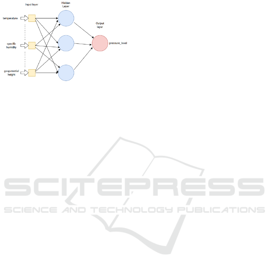
Figure 1: Systematic diagram of MLP: Depicting the inter-

connected layers responsible for feature selection and pre-

diction.

2.4 Advancements in ML Architectures

for Weather Forecasting

In “Spatio-temporal forecasting of weather and at-

tention mechanism on convolutional LSTMS”(Tekin

et al., 2021), Convolutional LSTM with Attention

Mechanisms was introduced as a hybrid architec-

ture combining context matchers and attention mech-

anisms with convolutional LSTM. MetNet(Sønderby

et al., 2020), Google Research’s neural weather

model, leverages ConvLSTM and axial attention pro-

cesses for high spatial and temporal resolution in

precipitation forecasting. MetNet outperforms lead-

ing operational weather forecasts based on NWP for

short-term predictions up to eight hours.

AIFS-ECMWF is a data-driven forecasting sys-

tem in which AIFS is a strong model providing proﬁ-

cient forecasts for upper-air variables, surface weather

parameters, and tropical cyclone tracks(Lang et al.,

2024). While effective, AIFS exhibits a slower im-

provement rate compared to the proposed MLP.

2.5 Optimizations and Challenges in

ML Forecasting Models

These ML models demonstrate the potential to over-

come the computational limitations of NWP by of-

fering high-resolution forecasts with reduced compu-

tational overhead. Research has also highlighted the

signiﬁcance of optimization strategies, including dy-

namic learning rate adjustments, regularization tech-

niques, and early stopping, in enhancing MLP perfor-

mance. With frameworks like TensorFlow and Keras,

these models have become more accessible, enabling

rapid prototyping and exploration of various architec-

tural conﬁgurations.

While ML models excel in handling short lead

times, they often face challenges with error prop-

agation as lead times increase. Additionally, cur-

rent models underutilize diverse data sources, such as

satellite imagery and ground-based observations, and

struggle to provide high-resolution forecasts within

reasonable computational constraints, especially for

global models. The proposed method addresses these

challenges by integrating pre-trained models tailored

for speciﬁc prediction periods, thereby reducing cu-

mulative errors and improving forecast accuracy for

both short and long lead times. By incorporating di-

verse datasets, including sensor observations, reanal-

ysis datasets, and satellite imagery, the approach cap-

tures complex weather dynamics comprehensively.

Innovative architectural designs strike a balance

between resolution and computational efﬁciency, en-

abling high-ﬁdelity forecasts with manageable re-

source requirements. This study advances ML-

based weather forecasting systems by providing ro-

bust methodologies for reliable, long-term, high-

resolution predictions, complementing or surpassing

traditional methods in various scenarios.

3 PROPOSED METHODOLOGY

This section details the methodology and techniques

employed in predicting weather forecasting using a

Multilayer Perceptron. A model fundamentally forms

a formula that, given a set of weights and their cor-

responding values attached to every training variable,

produces the target value(Jakaria et al., 2020). These

models are particularly useful in solving problems

where relationships among input features and target

variables exhibit complex non-linear forms. Weather

forecasting used a myriad of methodologies relying

on Genetic Algorithms and Neural Networks; yet, the

approaches used were insufﬁcient enough to capture

the intricate relationships between a myriad of factors

determining weather(Singh et al., 2019). For this re-

search, the implementation of the MLP utilized Ten-

sorFlow and Keras frameworks, which provide efﬁ-

cient design and training tools for neural networks.

These frameworks enable dynamic model archi-

tecture deﬁnitions and support systematic hyperpa-

rameter tuning through libraries like Keras Tuner.

This facilitates exploring parameters such as the num-

ber of layers, neurons per layer and the learning rate

to identify the optimal conﬁguration for weather pre-

diction. This process is divided into different stages:

data preprocessing, model design and training, evalu-

ation and metrics. In coordinates, we have date times-

tamps representing the temporal resolution. Pressure

levels in hectopascals (hPa), indicating vertical reso-

lution. Latitudes indicating Geographical north-south

axis (in degrees). Longitudes indicating Geographi-

INCOFT 2025 - International Conference on Futuristic Technology

362

cal east-west axis (in degrees). Version information

for data experiments (Expver).

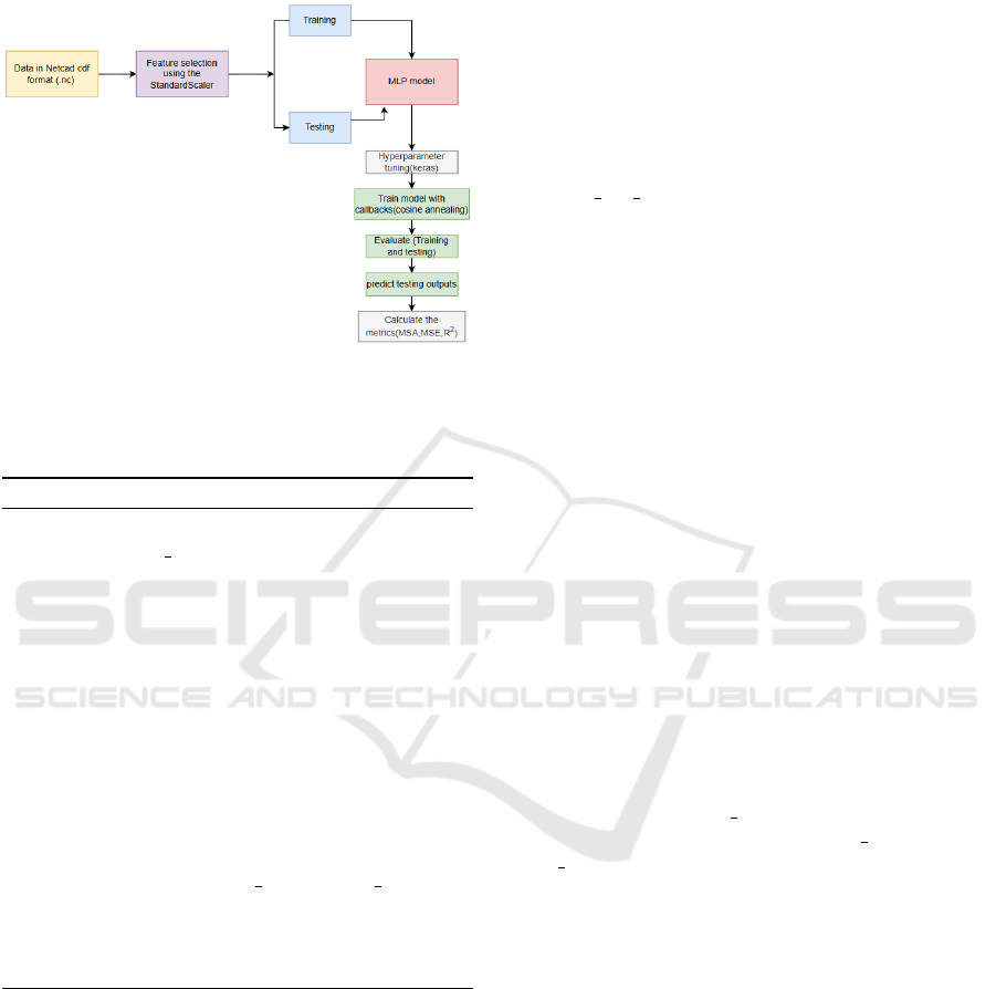
Figure 2: Workﬂow of the weather prediction model using

MLP.

3.1 Algorithmic Workﬂow

Algorithm 1 MLP Weather Data Modeling.

1: Load the weather dataset using

xarray.open mfdataset().

2: Extract relevant features: temperature, pressure,

and wind speed.

3: Handle missing values using fillna().

4: Normalize the dataset with StandardScaler().

5: Deﬁne the model using

tensorflow.keras.Sequential().

6: Compile the model with the adam optimizer and

mse loss function.

7: Split the data into training and testing sets.

8: Train the model using model.fit() with early

stopping and a cosine annealing scheduler.

9: Evaluate the model using

model.evaluate(test data, test labels).

10: Generate predictions using model.predict().

11: Compute mean absolute error (MAE) to compare

predictions with actual values.

We evaluate the model using metrics such as MSE in

ﬁg 4a, MAE in ﬁg 4b, and R-squared (R

) in ﬁg 4c on

both training and testing datasets.

3.2 Data Preprocessing

Data preprocessing involves several steps to prepare

the dataset for training the Multilayer Perceptron

model. Data Loading where ERA5 NetCDF(Zhong

et al., 2024) ﬁles are loaded using the xarray library,

which allows efﬁcient manipulation of multidimen-

sional data, such as pressure levels. A subset of the

data is extracted for computational efﬁciency, focus-

ing on pressure levels and other key features. Data

Cleaning where missing values in the dataset are han-

dled by either dropping them or imputing with sta-

tistical methods, such as mean imputation, to ensure

data consistency. Scaling where the StandardScaler

is used to normalize input features, improving the nu-

merical stability of to be standardized to have a mean

of 0 and a standard deviation of 1. Data Splitting by

dividing the dataset into training and testing sets us-

ingtrain test split, thus ensuring proper evaluation of

the model’s performance.

3.3 Feature Target Split

To predict atmospheric pressure levels as the target

variable, we performed a feature-target split on the

dataset. In the ﬁgure 2. Features used as inputs

(X) are atmospheric variables such as temperature (t),

horizontal and vertical wind components (Y), humid-

ity (r), and cloud cover (c). The target variable (Y),

which represents the vertical atmospheric pressure

level, was explicitly excluded from the feature set to

prevent data leakage. This manual feature selection is

a very direct and efﬁcient technique to ensure that the

model is only trained on the relevant predictor vari-

ables. By separating the target from the predictors,

we maintained the integrity of the predictive model-

ing process.

3.4 Scaling

Here, we manually select the relevant features in the

dataset to train our model. In this instance, the tar-

get variable, pressure level, is kept separate from

the rest of the features, such as feature 1 through fea-

ture 10. The columns remaining are the input to the

model. This is a straightforward form of feature se-

lection, where we explicitly exclude the target vari-

able from the dataset and use the remaining columns

as predictor features.

3.5 Implementation Approach

In MLP if labelled data are available, one may use

it as a training dataset from which to build a func-

tion that maps given inputs to outputs(Bochenek and

Ustrnul, 2022). Input Layer represents features in

the dataset, with each neuron representing one fea-

ture. Hidden Layer extracts patterns using fully con-

nected neurons and non-linear activation functions

like ReLU, enabling the model to learn complex rela-

tionships. Output layer produces the ﬁnal predictions.

In regression, it has one neuron with a linear activa-

Weather Forecasting Using Multilayer Perceptron Technique

363

tion for continuous outputs.

In the model training, the cosine annealing learn-

ing rate scheduler dynamically adjusts the learning

rate during training referring to the ﬁgure 2. It fol-

lows a cosine-shaped curve, starting from a maximum

learning rate, gradually decreasing, and then rising

slightly before restarting in the next cycle.

lr = lr

initial

× 0.5 ×



1 + cos



π ·

epoch%T

max



(1)

The cosine annealing technique modiﬁes in the

equation 1, the learning rate according to the train-

ing progress within a predetermined cycle T

max

. Low

learning rates (for ﬁne-tuning and convergence) and

high learning rates (for quick exploration of parame-

ter space) are seamlessly transitioned by it.

3.5.1 Metrics Calculation

MSE =

∑

i=1

− ˆy

)

(2)

The accuracy of the weather forecasting model is

assessed using the MSE 2. It restricts more severely

larger discrepancies between the predicted ˆy

and ac-

tual y

values since it squares the mistake. Extreme er-

rors, such as those in temperature or wind speed pre-

dictions, can be crucial in weather forecasting, there-

fore this is especially crucial. Here in the equation 2

n represents the sum of all observations, also known

as data points. This is a reference to the quantity of

weather forecasts under consideration. y

represents

the actual value that was observed in the ith instance.

ˆy

represents the expected value for the instance of

ith. For the same variable as y

, this is the value that

the weather forecasting model predicts. A low MSE

shows that the model can minimize signiﬁcant dis-

crepancies in predicted values, meaning that the pre-

dictions are close to the observed meteorological data.

MAE =

∑

i=1

− ˆy

| (3)

Another measure is MAE 3, which concentrates

on absolute differences rather than squaring them. It

is appropriate for assessing the average magnitude of

prediction mistakes since it is less susceptible to out-

liers than MSE. In the ﬁeld of weather forecasting,

MAE offers a more comprehensible indicator of the

average deviation between projections and actual ob-

servations. This measure makes sure that the forecast-

ing system operates consistently in all situations and

isn’t unduly impacted by excessive errors. n denotes

the total number of observations, much like in MSE 2.

for the ith instance, is the actual observed value. ˆy

is the anticipated value for the occurrence of ith

= 1 −

residual

ss total

(4)

The model’s goodness-of-ﬁt is assessed using R

as 4. It calculates the ratio of the observed data’s vari-

ance (y

) to that of the model’s predictions (ˆy

). A

high-quality model is suggested by R

value nearer

1, which shows that the model accounts for the ma-

jority of the variability in the meteorological data.

Lower values, on the other hand, would suggest that

the model has trouble identifying patterns in the data.

residual

∑

i=1

− ˆy

)

(5)

Equation 5 gives the residual sum of squares. This

is the overall squared error for all data points between

the observed and anticipated values. It is the equa-

tion’s numerator and shows how much variance the

model is unable to account for.

total

∑

i=1

− ¯y)

(6)

Equation 6 gives the total sum of squares. By cal-

culating the squared differences between the observed

values and their mean ¯y, this sums up the variance in

the observed data y

3.6 Challenges and Solutions

In the absence of techniques such as hyperparameter

tuning, Adam W optimizer and cosine annealing

scheduler optimization, we were obtaining test and

train accuracies that were identical, with not even

a decimal point difference. We discovered a differ-

ence between them after utilizing hyperparameter

adjustment, the Adam W optimizer, the cosine

annealing scheduler, and deepening the MLP with

train accuracy present in the table ?? MSE 56.3173,

MAE 5.4549 and R² 0.9991 and the test accuracy

as MSE 91.9154, MAE 7.0193 and R² 0.9985. The

dataset contained inconsistent rows, which could

cause errors in the analysis. Furthermore, there was a

large search space for hyperparameter optimization,

which made it challenging to quickly ﬁnd the ideal

combination. The last problem was overﬁtting, which

occurred when the model appeared to memorize the

training data instead of effectively generalizing to

new data.

In order to resolve the problem of inconsistent

rows, we either eliminated rows with missing data or,

when practical, ﬁlled in the missing values, keeping

INCOFT 2025 - International Conference on Futuristic Technology

364

the dataset accurate and clean. We employed keras-

tuner to address the intricate issue of hyperparameter

tuning, which aided in automating and streamlining

the search procedure, increasing its effectiveness and

focus. We used early stopping to prevent overﬁtting,

which uses validation splitting to track performance

on unseen data during training and stops training

when the model’s performance begins to deteriorate

on the validation set. These tactics made sure the

model stayed strong and had good generalization

capabilities.

4 RESULTS AND ANALYSIS

This dataset serves as a crucial resource for under-

standing key concept of the weather forecasting. It

is available in the NetCDF format, retrieved from the

hourly ERA5 pressure level data provided by the Eu-

ropean Centre for Medium-Range Weather Forecasts

(ECMWF). It spans 36 months, from January 2021 to

September 2024, sampled monthly, and includes two

pressure levels (1000 hPa and 500 hPa). It covers a

latitude range from 90.0° to -90.0° and a longitude

range from 0.0° to 359.75°, both in 0.25° intervals.

Coordinates include timestamps representing tempo-

ral resolution, pressure levels indicating vertical res-

olution, and geographical north-south (latitude) and

east-west (longitude) axes, with version information

for data experiments (expver).

The Dataset has 36 timestamps (date), 2 pressure

levels, 721 latitude points, and 1440 longitude points.

It has 16 atmospheric variables including tempera-

ture, in general, can be measured to a higher degree

of accuracy relative to any of the other weather vari-

ables(Tektas¸, 2010), wind components, relative hu-

midity, ozone concentration, and different cloud prop-

erties. The variables are stored in multidimensional

arrays indexed by time, pressure level, latitude, and

longitude in the ﬂoat32 format. The NetCDF format

ensures storage and access efﬁciency for the multi-

dimensional data, permitting slicing and aggregation

operations. Metadata follows CF-1.7 conventions and

outlines information about the source, institution, and

experiment version of the data. Thus, this dataset is

adequate for weather forecasting and modeling atmo-

spheric conditions. Here with an R2 value of 0.9991,

the MLP conquers numerous conﬁnements of the sin-

gle layer perceptron (Shamshad et al., 2019) MLP

demonstrated great accuracy during training, explain-

ing almost all of the variance in the target variable.

Strong generalization abilities are demonstrated on

the test set by the R2 of 0.9985, despite somewhat

higher MSE and MAE, which indicate slight overﬁt-

ting. The outcomes conﬁrm that optimization meth-

ods such as cosine annealing and AdamW are able to

improve learning and avoid overﬁtting. The Adam

is a stochastic method of optimization, which uses

an idea of gradient descent combined with the con-

cept of momentum toward minimizing the loss func-

tion and also ﬁnd the minimum value of its function.

A comparative analysis of the proposed MLP model

against state-of-the-art approaches (AIFS ,FuXi ,Met-

Net , and ConvLSTM) reveals the following:

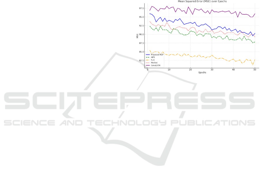
Figure 3: Line graph showing the model performance in

epochs.

The line graph in ﬁg 3 shows the models’ per-

formance over 50 epochs in terms of MSE ﬁg 4a.

Proposed MLP shows consistent progress, achieving

competitive MSE values at training’s conclusion. Af-

ter referring to the table 1 we can see that AIFS

maintains a strong overall performance but exhibits a

somewhat slower rate of improvement as compared to

the proposed MLP. FuXi consistently performs well

throughout, achieving the best MSE values. MetNet

a little better than AIFS and FuXi, but with a some-

what higher MSE. ConvLSTM has the greatest MSE

at the conclusion of each epoch and the slowest MSE

reduction. Although AIFS requires a lot of process-

ing power for training, its use of sophisticated GNNs

and attention mechanisms makes it highly ﬂexible and

scalable to big datasets.

The models’ development during training is seen

in this visualization. The AIFS model outperforms

the suggested MLP by a small margin on these met-

rics, with an MSE of 88.0 and an MAE of 6.85. Ad-

vanced GNN and transformer-based designs are two

advantages of AIFS that help explain its excellent ac-

curacy with the best MSE (70.32) and MAE (6.12),

the FuXi model performs better when it comes to gen-

eralizing over long-term weather forecasts. Both the

Proposed MLP and the MetNet model have compet-

itive MSE and R

values. Nonetheless, the empha-

sis placed by MetNet on high-resolution precipitation

forecasts might marginally diminish its overall gen-

Weather Forecasting Using Multilayer Perceptron Technique

365

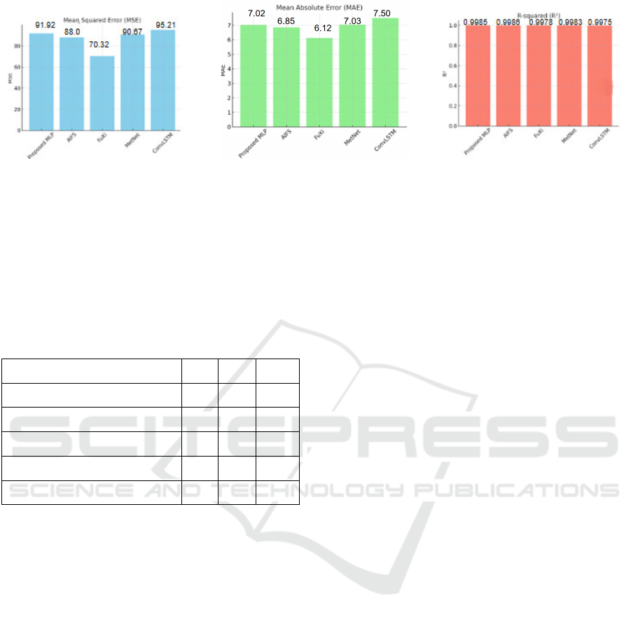
(a) Figure 4.a (b) Figure 4.b (c) Figure 4.c

Figure 4: Visualization showing the performance of different models during training.

erality. The Proposed MLP (R

= 0.9985) comes in

second to the AIFS model, which has the greatest R

(0.9986). This indicates that nearly all of the volatility

in the data can be explained by both models. MetNet

performs admirably as well (R

= 0.9983), lagging the

proposed MLP by a small margin.

Table 1: Performance metrics for training and testing

datasets.

Model MSE MAE R

AIFS (Lang et al., 2024) 88.0 6.85 0.9986

FuXi (Chen et al., 2023) 70.32 6.12 0.9978

MetNet (Sønderby et al., 2020) 90.67 7.03 0.9983

ConvLSTM (Tekin et al., 2023) 95.21 7.50 0.9975

Proposed MLP 91.92 7.02 0.9985

Although AIFS needs enormous computational power

for training it is highly ﬂexible and scalable with big

datasets due to the use of complex GNNs and atten-

tion mechanisms. The previous study further pro-

poses to represent weather by the use of hierarchi-

cal features which are learned from large amounts of

weather data through DNN.(Salman et al., 2015). Ad-

vantage, which is suitable for medium-range forecast-

ing applications.

ANN has advantages over other weather forecast-

ing techniques in that the ANN minimizes the error

with a variety of algorithms and gives us a predicted

value which is nearly equal to the actual value. (Ab-

hishek et al., 2012). The Proposed MLP is more

approachable due to its more straightforward archi-

tecture, which strikes a balance between competitive

accuracy and computing economy. In the Bar chart

3AIFS dominates the analysis by striking a compro-

mise between scalability for big datasets and excel-

lent accuracy (lowest MSE and highest R²). Its pro-

cessing needs, however, are much greater. For long-

term forecasting, the optimal option for 15-day fore-

casts is FuXi, which has the lowest MSE and MAE.

Sometimes a very low MSE can be mistaken as good

accuracy when in fact it points to a serious prob-

lem called ‘overﬁtting’(Abhishek et al., 2012). In the

ﬁgure 4, the results indicate that MLPs are suitable

for deployment in real-world systems and validate

their feasibility for precise weather prediction tasks

with lower scores indicating more successful predic-

tions.(Sha et al., 2024)

5 CONCLUSIONS

By creating an accurate and effective MLP based

model for predicting atmospheric pressure levels, this

work addressed the shortcomings of conventional

forecasting techniques. It achieved high R2 values

of 0.9991 (training) and 0.9985 (testing). A weather

forecast is crucial for the outcome and understanding

all the processes that lead to the outcome and chang-

ing environment.(Inness and Dorling, 2012) Accu-

racy, strong generalization, and less overﬁtting were

guaranteed by methods like cosine annealing, hy-

perparameter optimization, and the AdamW opti-

mizer.(Llugsi et al., 2021) In medium-range weather

forecasting, the model performed better than tradi-

tional methods, providing increased efﬁciency and

accuracy. Forecasts can be used to plan activities

around these events and to plan ahead and survive

them(Narvekar and Fargose, 2015). Future research

might concentrate on improving hyperparameters,

adding factors like precipitation, integrating hybrid

models for long-term projections, growing datasets,

and creating useful tools for uses like disaster relief.

REFERENCES

Abhishek, K., Singh, M. P., Ghosh, S., and Anand, A.

(2012). Weather forecasting model using artiﬁcial

INCOFT 2025 - International Conference on Futuristic Technology

366

neural network. Procedia Technology, 4:311–318.

Bochenek, B. and Ustrnul, Z. (2022). Machine

learning in weather prediction and climate analy-

ses—applications and perspectives. Atmosphere,

13(2):180.

Bushara, N. O. and Abraham, A. (2014). Weather forecast-

ing in sudan using machine learning schemes. Journal

of Network and Innovative Computing, 2:9–9.

Chen, L., Zhong, X., Zhang, F., Cheng, Y., Xu, Y., Qi, Y.,

and Li, H. (2023). Fuxi: A cascade machine learning

forecasting system for 15-day global weather forecast.

npj Climate and Atmospheric Science, 6(1):190.

Fente, D. N. and Singh, D. K. (2018). Weather forecasting

using artiﬁcial neural network. In 2018 Second Inter-

national Conference on Inventive Communication and

Computational Technologies (ICICCT), pages 1757–

1761. IEEE.

Inness, P. M. and Dorling, S. (2012). Operational weather

forecasting. John Wiley & Sons.

Jakaria, A., Hossain, M. M., and Rahman, M. A.

(2020). Smart weather forecasting using machine

learning: A case study in tennessee. arXiv preprint

arXiv:2008.10789.

Jaseena, K. and Kovoor, B. C. (2022). Deterministic

weather forecasting models based on intelligent pre-

dictors: A survey. Journal of King Saud University

- Computer and Information Sciences, 34(6):3393–

3412.

Kothapalli, S. and Totad, S. (2017). A real-time weather

forecasting and analysis. In 2017 IEEE International

Conference on Power, Control, Signals and Instru-

mentation Engineering (ICPCSI), pages 1567–1570.

IEEE.

Lang, S., Alexe, M., Chantry, M., Dramsch, J., Pin-

ault, F., Raoult, B., Clare, M. C., Lessig, C.,

Maier-Gerber, M., Magnusson, L., et al. (2024).

Aifs-ecmwf’s data-driven forecasting system. arXiv

preprint arXiv:2406.01465.

Llugsi, R., El Yacoubi, S., Fontaine, A., and Lupera, P.

(2021). Comparison between adam, adamax and

adamw optimizers to implement a weather forecast

based on neural networks for the andean city of

quito. In 2021 IEEE Fifth Ecuador Technical Chap-

ters Meeting (ETCM), pages 1–6. IEEE.

Medar, R., Angadi, A. B., Niranjan, P. Y., and Tamase, P.

(2017). Comparative study of different weather fore-

casting models. In 2017 International Conference

on Energy, Communication, Data Analytics and Soft

Computing (ICECDS), pages 1604–1609. IEEE.

Narvekar, M. and Fargose, P. (2015). Daily weather fore-

casting using artiﬁcial neural network.

Salman, A. G., Kanigoro, B., and Heryadi, Y. (2015).

Weather forecasting using deep learning techniques.

In 2015 International Conference on Advanced Com-

puter Science and Information Systems (ICACSIS),

pages 281–285. IEEE.

Sha, Y., Sobash, R. A., and Gagne, D. J. (2024).

Generative ensemble deep learning severe weather

prediction from a deterministic convection-allowing

model. Artiﬁcial Intelligence for the Earth Systems,

3(2):e230094.

Shamshad, B., Khan, M. Z., and Omar, Z. (2019). Mod-

eling and forecasting weather parameters using ann-

mlp, arima and ets model: A case study for lahore,

pakistan. International Journal of Scientiﬁc & Engi-

neering Research, 10(4):351–366.

Singh, N., Chaturvedi, S., and Akhter, S. (2019). Weather

forecasting using machine learning algorithm. In 2019

International Conference on Signal Processing and

Communication (ICSC), pages 171–174. IEEE.

Sønderby, C. K., Espeholt, L., Heek, J., Dehghani, M.,

Oliver, A., Salimans, T., Agrawal, S., Hickey, J., and

Kalchbrenner, N. (2020). Metnet: A neural weather

model for precipitation forecasting. arXiv preprint

arXiv:2003.12140.

Tekin, S. F., Karaahmetoglu, O., Ilhan, F., Balaban, I., and

Kozat, S. S. (2021). Spatio-temporal weather forecast-

ing and attention mechanism on convolutional lstms.

arXiv preprint arXiv:2102.00696, 4.

Tektas¸, M. (2010). Weather forecasting using anﬁs and

arima models. Environmental Research, Engineering

and Management, 51(1):5–10.

Zhong, X., Chen, L., Li, H., Liu, J., Fan, X., Feng,

J., Dai, K., Luo, J.-J., Wu, J., and Lu, B. (2024).

Fuxi-ens: A machine learning model for medium-

range ensemble weather forecasting. arXiv preprint

arXiv:2405.05925.

Weather Forecasting Using Multilayer Perceptron Technique

367