Denoising Synthetic Aperture Radar / Aerial Images Using HOTV Deep
Learning Models with Bayesian MAP Approach
Ashok Shrimant Hake
1
, Krishnendu Remesh
2
a
and Vishal Subhas h Chavan
1
1
Dept. of Computer Science and Business Systems, KIT’s College of Engineering Kolhapur, Maharashtra, India
2
Department of Mathematics, Christ University, Bengaluru, Karnataka, India
Keywords:
Image Denoising, Total Variation Model, HOTV, CNN Model.
Abstract:
Denoising plays an essential role in Synthetic Aperture Radar (S A R) and aerial image restoration. These
images are distorted with various noises due to atmospheric changes. Therefore, the images should be analyzed
using proper restoration and enhancement techniques. Many authors proposed traditional and deep learning
models to perform this task. This paper employed the Bayesian Maximum A Posteriori (MAP) approach to
the Higher Order Total Variat ion (HOTV) deep learning model. We assumed that the Poisson noise distorts
the images. We also used the model t o restore the images degraded by noises such as Gamma, Gaussian, and
Rayleigh. Quantitative and qualitative analyses are provided.
1 INTRODUCTION
A wide variety of noise an d distortions, including
blur, decreased contrast, intensity, and inhomogen e -
ity, frequently deteriorate sen sor da ta Rasti et al.
(2021). One of the primary causes of the deteriora-
tion of satellite, remote-sensed, and aerial images is
the presence of several types of noise. Poisson noise
is one of the most common noises in Synthetic Aper-
ture Radar (SAR) images, and this type of noise ulti-
mately increases the difficulty of interpreting images
Febin et al. ( 2020) .
A noisy satellite or aerial image can be formulated
by
x
0
= x ∗ n, (1)
where x represents the original imag e, while n denotes
the multiplicative noise, which is observed to follow
a Poisson distribution. Mathematically, the denoisin g
problem of the images is ill-p osed.
Many studies have been carried out in denoising
the images. The models employed local filters that
could not retain essential details, such as edges, due to
the assumption that neighboring pixels shared identi-
cal statistical characteristics Rasti et al. (2021). No n-
local models estimate the weighte d non-local similar-
ity between small image patches to preserve resolu-
tion while removing the noise. Many othe r authors
a
https://orcid.org/0000-0001-6713-8483
have used non-local denoising models for SAR im-
ages Deledalle e t al. (2014); Parrilli et al. (2011).
Total Variatio nal (TV) Model (Rudin Osher
Fatemi (ROF) model) are well known for image de-
noising Rudin et al. (1992). TV-based models are effi-
cient because of their a bility to preserve edges. How-
ever, the staircase effect is the main flaw in the TV-
based method Strong and Chan (2003). The optimiza-
tion fu nction in the TV model is a trade-off betwee n
data fidelity and regularization. It is formulated by:
min
x
λ
2
kx
0
− xk
2
2
+ k∇xk
1
, (2)
where λ > 0 and x is the original ima ge or de sired
image. Even though the large values of λ retain the
features in the images, the small values of λ provide
better denoising. Therefore, a n optimal choice of λ is
mandatory.
Many modified approaches to TV model Li and
Li (2021) have been propo sed to rectify the stair-
case effect. By considering the h igher-order gradient,
the Higher-Order Total Variation model is introduced
Lysaker et al. (2003). It is formulated by:
min
x
λ
2
kx
0
− xk
2
2
+ k∇
2
xk
1
. (3)
The higher order gradient with the L
1
norm reduces
the staircase effect of the regular TV model in the im -
age restoration.
Aubert and Aujol introduced a Bayesian Maxi-
mum A Posteriori (MAP) model using MAP estima-
662
Hake, A. S., Remesh, K. and Chavan, V. S.
Denoising Synthetic Aperture Radar / Aerial Images Using HOTV Deep Learning Models with Bayesian MAP Approach.
DOI: 10.5220/0013599700004664
Paper published under CC license (CC BY-NC-ND 4.0)
In Proceedings of the 3rd International Conference on Futuristic Technology (INCOFT 2025) - Volume 2, pages 662-668
ISBN: 978-989-758-763-4
Proceedings Copyright © 2025 by SCITEPRESS – Science and Technology Publications, Lda.

tor with the total variation regularization in Aubert
and Aujol (2008). The model facilitates handlin g
multiplicative gamma noise. While effective to some
extent, traditional models may struggle to handle
complex noise patterns and may introduce undesir-
able artifacts in the denoised image s.
Deep learning models CNNs to ada pt the relation
between clean and noisy images. By leveraging
large datasets and learning complex patterns directly
from data, CNNs have demonstrated remarkable
performance in various image denoising Jebur et al.
(2024). These models are widely studied in SAR
image de noising also. Chierchia et al. proposed a
residual-ba sed learning model in Chierchia et al.
(2017), which has a faster convergence. However,
Training involves using a large multitemporal SAR
image to approximate a clean image. A Bayesian
despeckling method in spired by blind-spot denoising
networks and incorporating a TV regularizer is
employed by Molini et al. in Molini et al. (2021).
We conside r a CNN model based on Bayesian MAP
approa c h.
2 DATA FIDELITY TERMS USING
BAYESIAN MAP
According to Bayesian rule,
P(U|V) =
P(V |U )P(U)
P(V )
, (4)
where P(U|V ) is the cond itional probability of the
random variable U given V. Here, we use the ab ove
Bayesian rule and try to restore the image by maxi-
mizing the posterior probability P(x|x
0
) given by
P(x|x
0
) =
P(x
0
|x)P(x)
P(x
0
)
. (5)
That is,
max
x
P(x|x
0
) = max
x
P(x
0
|x)P(x), (6)
The term P(x
0
), the prior probability on x
0
, is a con-
stant w.r.t. x that can be neglected.
Assume that the speckles in SAR images follow
the Poisson noise. Therefore, the posterior probability
function P(x
0
|x) is given as
P(x
0
|x) =
exp(−x)x
x
0
x
0
!
(7)
One can consider th e ima ge (x and x
0
) as a set of
indepen dent pixels of the imag e , say x
i
, (The joint
probability equals the product of the marginal prob-
abilities of each random variable x(x
i
)), therefore, (6)
can be w ritten as
max
x
P(x(x
i
)|x
0
(x
i
)) = max
x
N
∏
i=1
P(x
0
(x
i
)|x(x
i
))P(x(x
i
)),
(8)
where N is the total number of image samples.
Since the function log is a m onoton e function,
maximizing P(x|x
0
) is equivalent to minimizing the
negative log-likelihood, and hence from (7) a nd (8),
we can obtain the following;
min
x
(
N
∑
i=1
x(x
i
)−x
0
(x
i
)log(x(x
i
))−
N
∑
i=1
log(P(x(x
i
)))
)
(9)
where the prior of x, say P(x), follows a regularization
prior. For the sake of simplicity, we eliminate x
i
, thus
we get,
min
x
{−logP(x|x
0
)} = min
x
(
x − x
0
logx + λφ(x)
)
,
(10)
where φ(x) be the pr ior probability function. Many
authors considered φ(x) is the the total variation of x.
3 MAP MODEL WITH HOTV
REGULARIZATION
We implemented a deep lea rning model using a Con-
volutional Neural Network (CNN) arch itecture de-
signed for Higher Orde r Total Variation (HOTV).
Generally, we use th e loss function of the HOTV
model as in (3). In this paper, we designed the model
for the loss function Poisson + HOTV which works
well to restor e the SAR/Ariel images disto rted with
the poisson noise. We consider the objective function
as in (10) with the assumption that the prior prob-
ability φ(x) f ollows HOTV, provide d the noise fol-
lows the Poisson distribution. That is, the fidelity
term is x − x
0
logx and the prior regularizatio n of x is
φ(x) = k∇
2
xk
1
.
Also, we consider the model feature a cu stom loss
function that integrates the HOTV loss function with
other loss functions’ Bayesian approach to address
different noise types. So the model can be ea sily
adapted to han dle other no ise distributions, such as
Gamma, Gaussian, and Rayleigh, by modifyin g the
data fidelity term. We experimented with the model
with three variations of loss functions: Gamma +
HOTV, Gaussian + HOTV, and Rayleigh + HOTV. By
employing the same architecture and dataset of orig-
inal images, we evaluated the performance of these
Denoising Synthetic Aperture Radar / Aerial Images Using HOTV Deep Learning Models with Bayesian MAP Approach
663

combined loss function models to determine their ef-
fectiveness in denoising. Note tha t, we used the spe-
cific loss function to reconstruct the image distorted
by the corresponding noise.
We consider th e data fidelity terms according to
the nature of noise (see Table I) along with the fixed
prior regularization ter m. Note that the Gaussian
noise is a dditive.
Table 1: Data Fidelity Term for Various Noises.
Noise D istribution Data Fidelity Term
Gamma logx +
x
0
x
Gaussian (x − x
0
)
2
Rayleigh 2log(x)+
x
2
0
2x
3.1 Model Architecture
The deep learning m odel employed for HOTV uti-
lized a CNN architecture. The details of the mo del
layers, output shapes, and p arameters are given in Ta-
ble II. We use a total of 121,355 parameters such that
40,451 trainable paramete rs and 80,904 Optimizer pa-
rameters.
Table 2: Model architecture with layer details, output
shapes, and parameter counts.
Layer (type) Output
Shape
Param #
conv2d
(Conv2D)
(None, 256,
256, 64)
1,792
conv2d 1
(Conv2D)
(None, 256,
256, 64)
36,928
conv2d 2
(Conv2D)
(None, 256,
256, 3)
1,731
3.2 Hyperparameters and Training
Configuration
We consider the Adam optimizer with a learning rate
of 0.0 01 for all the models except the Rayleigh +
HOTV model. For the Rayleigh model, the learning
rate considered 0.0001 for better perfor mance and im-
proved quality metrics. We use the ReLU activatio n
function for the first two convolutional layer s and Sig-
moid for the final convolutional layer. The λ value
for balancing the regularization term with the data fi-
delity term in the HOTV loss function is set to 0.0001.
The models were trained using a dataset consisting of
2000 aerial images.
Algorithm 1 Training and Evaluation of I mage De-
noising Models
1: Input: Noisy images X , Clean images Y , Num-
ber of epochs E, Batch size. B
2: Output: Trained mo del, Evaluation metr ic s.
3: Initialize model parameters.
4: Define the combined loss function as in (10).
5: for each model type do
6: Compile th e model with Adam optimizer and
loss function.
7: for epoch = 1 to E do
8: Shuffle the training data.
9: for batch = 1 to N/B do
10: Select a batch of noisy images X
batch
and clean images Y
batch
.
11: Perform forward pass to compute pre-
dictions
ˆ
Y
batch
.
12: Compute loss using the combined loss
function.
13: Perform backward pass to update
model parameters.
14: end for
15: end for
16: Save the trained model.
17: Evaluation:
18: for each test image do
19: Load noisy image X
test
and corresponding
clean image Y
test
.
20: Denoise the image using the trained
model to get
ˆ
Y
test
.
21: Compute evalu ation metrics (MSE,
PSNR, SSIM).
22: Store the computed metrics.
23: end for
24: Save evaluation metrics to an Excel file.
25: end for
4 QUANTITATIVE AND VISUAL
ANALYSIS
To evaluate the performance of our de e p lear ning-
based image denoising models, we assessed them us-
ing three standard quality metrics: Mean Squared Er-
ror (MSE), Peak Signal-to-Noise Ratio (PSNR), and
Structural Similarity Index (SSIM). These metrics
provide a comprehensive evaluation of ima ge quality
and denoising effectiveness.
MSE measures the average squared difference b e-
tween the noisy and denoised images, with lower val-
ues indicating better performance. Th e PSNR quanti-
fies the ratio of th e maximum possible signal power to
the noise power, with higher values signifying better
INCOFT 2025 - International Conference on Futuristic Technology
664

quality. It is formulated as
PSNR = 10 .log

x
2
max
MSE

,
where x
max
denotes the maximum pixel intensity. A
higher PSNR value (in dB) indic ates better ima ge
quality. SSIM is defined as
SSIM(x, x
0
) =
(2µ
x
µ
x
0
+ c
1
)(2σ
x
0
+ c
2
)
(µ
2
x
µ
2
x
0
+ c
1
)(σ
2
x
+ σ
2
x
0
+ c
2
)
,
where µ
x
,µ
x
0
are the means and σ
x
,σ
x
0
are the vari-
ances of x,x
0
, respectively. The variables c
1
and
c
2
stabilize the division with a weak d enominator.
SSIM assesses the similarity between the original and
denoised images, with values closer to 1 in dicating
higher similarity. The following tables present the de-
tailed quality metrics for various noise models applied
in our study.
Table 3: Quality Metrics for Poisson + HOTV Model
Image MSE PSNR
(dB)
SSIM
img1 8.2905 38.846 0.9932
img2 10.4559 36.068 0.9828
img3 3.6985 42.432 0.9933
img4 4.8233 41.280 0.9921
img5 5.5569 40.646 0.9830
img6 3.6464 42.494 0.9939
img7 4.9850 41.147 0.9933
img8 13.4772 35.860 0.9883
img9 3.2891 42.945 0.9916
img10 4.7166 41.313 0.9939
Average 6.0652 40.469 0.9890
Table 4: Quality Metrics for Standard HOTV Model
Image MSE PSNR
(dB)
SSIM
img1 33.93 32.40 0.847
img2 39.90 31.20 0.972
img3 24.11 33.87 0.865
img4 50.55 29.60 0.963
img5 18.27 35.42 0.968
img6 22.56 34.01 0.933
img7 26.78 33.12 0.912
img8 20.34 34.58 0.941
img9 29.45 32.78 0.918
img10 31.56 32.54 0.906
Average 29.50 32.74 0.927
Table 5: Quality Metrics for Gamma + HOTV Model
Image MSE PSNR
(dB)
SSIM
img1 11.45 37.50 0.958
img2 24.00 33.77 0.916
img3 23.89 33.86 0.910
img4 34.17 32.30 0.912
img5 22.97 33.93 0.925
img6 12.34 36.92 0.946
img7 28.56 32.98 0.904
img8 19.43 34.71 0.929
img9 15.67 35.83 0.939
img10 21.12 34.24 0.921
Average 22.23 34.29 0.922
Table 6: Quality Metrics for Gaussian + HOTV Model
Image MSE PSNR
(dB)
SSIM
img1 52.12 29.05 0.891
img2 32.24 31.71 0.801
img3 54.43 29.13 0.795
img4 34.56 32.32 0.823
img5 39.51 31.48 0.835
img6 45.67 30.28 0.812
img7 38.29 31.52 0.804
img8 47.12 30.17 0.829
img9 43.67 30.76 0.845
img10 51.34 29.29 0.820
Average 43.39 30.70 0.818
Table 7: Quality Metrics for Rayleigh + HOTV Model
Image MSE PSNR
(dB)
SSIM
img1 47.6392 30.178 0.8298
img2 68.1799 28.234 0.8519
img3 117.3053 17.346 0.8055
img4 31.1744 31.814 0.8541
img5 61.6765 28.565 0.9192
img6 57.8432 29.310 0.8999
img7 80.7006 26.937 0.8610
img8 66.2137 27.874 0.9063
img9 41.7139 31.200 0.8537
img10 71.9193 28.108 0.8612
Average 65.5326 27.786 0.8740
5 CONCLUSION
In conclusion, the HOTV + Poisson mode l is the most
effective in preserving image qu ality and reducing
noise, while the other models, demonstrate varying
degrees of effectiveness and quality trade-offs. Pois-
Denoising Synthetic Aperture Radar / Aerial Images Using HOTV Deep Learning Models with Bayesian MAP Approach
665

son + HOTV Model exhibits the highest overall per-
formance with an average MSE of 6.0652, indicat-
ing superior noise reduction. It a chieves th e high-
est average PSNR of 40.469 and SSIM of 0. 9890,
demonstra ting excellent preservation of image qual-
ity and structural similarity. These results highlight
its effectivene ss in produc ing high-fidelity deno ised
images. Also, Gamma + HOTV model demonstrates
moderate performance when the images are distorted
with Gamma noise. It provides a balanced approach
to noise reduction and image fide lity but do es not
achieve the superior qu ality seen with the Poisson
model. The standard HOTV model, also strikes a bal-
ance between effective noise reduction and maintain-
ing image quality, though it does not reach the level
of performan c e achieved by the Poisson model. The
other two models indicate a loss in image quality and
noticeable distortions.
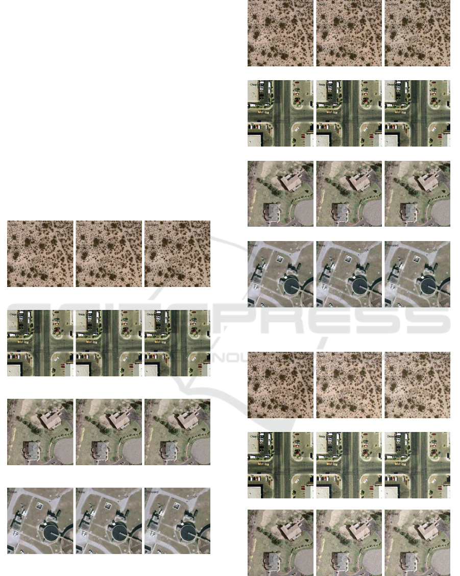
Figure 1: Denoising results for Poisson + HOTV Model
with Poisson Noise. In each figure, the first image is clean,
the second is noisy and the third is restored.
Figure 2: Denoising results for Standard HOTV Model with
Speckle Noise. In each fi gure, the first image is clean, the
second is noisy, and the third is restored.
INCOFT 2025 - International Conference on Futuristic Technology
666

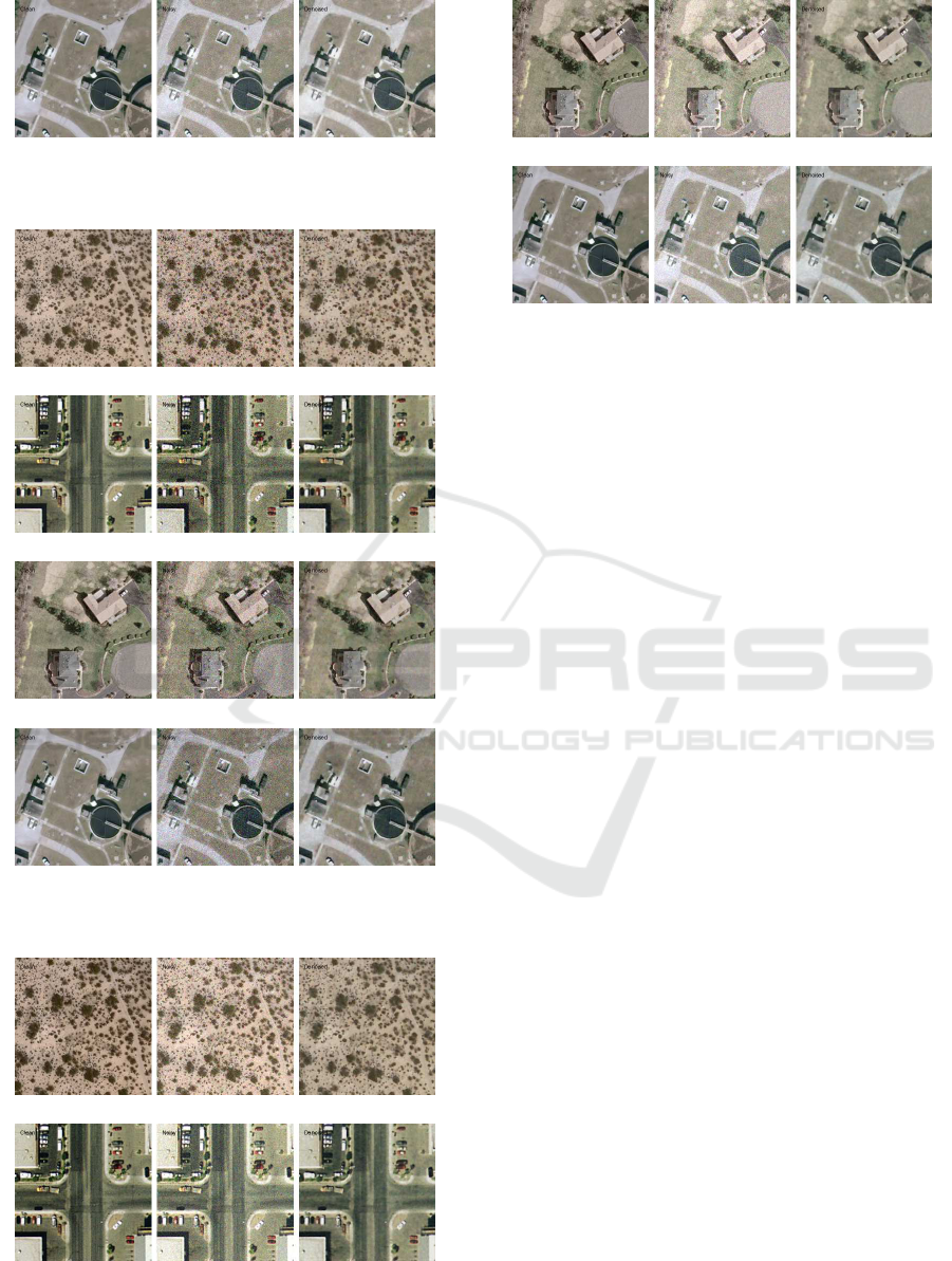
Figure 3: Denoising results f or Gamma + HOTV Model
with Gamma Noise. In each figure, the fir st i mage is clean,
the second is noisy, and the third is restored.
Figure 4: Denoising results for Gaussian + HOTV Model
with Gaussian Noise. In each figure, the first image is clean,
the second is noisy, and the third is restored.
REFERENCES
Aubert, G. and Aujol, J.-F. (2008). A variational ap -
proach to removing multiplicative no ise. SIAM
Figure 5: D enoising results for Rayleigh + HOTV Model
with Gaussian Noise. In each figure, the first image is clean,
the second is noisy, and the third is restored.
journal on applied mathematics, 68(4):925–946.
Chierchia, G., Coz zolino, D., Poggi, G., and Verdo-
liva, L. (2017). Sar image despeckling through
convolutional neural networks. In 2017 IEEE in-
ternational geoscience and remote sensing sym-
posium (IGARSS), pages 5438–5441. IEEE.
Deledalle, C.-A., Denis, L., Tupin, F., Reigber, A.,
and J¨ager, M. (2014). Nl-sar: A unified nonlocal
framework for resolu tion-preser ving ( pol)(in)
sar denoising. IEEE Transactions on Geoscience
and Remote Sensing, 53(4):2021– 2038.
Febin, I., Jidesh, P., and Bini, A. (2020 ). A retinex-
based variational model for enhancem ent and
restoration of low-contrast remote-sensed im-
ages co rrupted by shot noise. IEEE Journal of
Selected Topics in Applied Earth Observations
and Remote Sensing, 13:941–949.
Jebur, R. S., Zabil, M. H. B. M ., Hamm ood, D. A.,
and Cheng, L. K. (2024). A comprehensive re-
view of image denoising in deep learning . Mul-
timedia Tools and Applications, 83(20):58181–
58199.
Li, M.-M. and Li, B.-Z. (2021). A novel weighted
total variation model for image denoising. IET
image processing, 15(12):2749–2760.
Lysaker, M., Lundervold, A., and Tai, X.-C. (2003).
Noise rem oval using fourth-order par tial dif-
ferential equ ation with applications to medi-
cal mag netic resonance images in space and
time. IEEE Transactions on image processing,
12(12):1579–1590.
Molini, A. B., Valsesia, D., Fracastoro, G., and Magli,
E. (2021). Speckle2void: Deep self-supervised
sar despeckling with blind-spot convolutional
neural networks. IEEE Transactions on Geo-
science and Remote Sensing, 60:1–1 7.
Parrilli, S., Poderico, M., Angelino, C. V., and Verdo-
Denoising Synthetic Aperture Radar / Aerial Images Using HOTV Deep Learning Models with Bayesian MAP Approach
667

liva, L. (2011) . A nonlocal sar image d enoising
algorithm based on llmmse wavelet shrinkage.
IEEE Transactions on Geoscience and Remote
Sensing, 50(2):606–6 16.
Rasti, B., Chang, Y., Dalsasso, E., Denis, L.,
and Ghamisi, P. (2021). Image restoration
for remote sensin g: Overview and toolbox.
IEEE Geoscience and Remote Sensing Maga-
zine, 10(2):201–230.
Rudin, L. I., Osher, S., and Fatemi, E. (1992). Non-
linear total variation based noise removal algo-
rithms. Physica D: nonlinear phenomena, 60(1-
4):259–268.
Strong, D. and Chan, T. (2003). Edge-preserving and
scale-depen dent properties of total variation reg-
ularization. Inverse problems, 19(6):S165.
INCOFT 2025 - International Conference on Futuristic Technology
668