Cognitive Load Classification Using Feature Masked Autoencoding

and Electroencephalogram Signals

D. Eesha

1,2

, M. Nagaraju

1,2

, D. Divya

1,2

and S. Kashyap Reddy

1,2

Institute of Aeronautical Engineering, Hyderabad, Telangana, India

Department of CSE(AI&ML), Institute of Aeronautical Engineering, Hyderabad, Telangana, India

Keywords: Cognitive Load, Deep Learning, EEG Data, Load Classification, Machine Learning, Masked Autoencoder

Abstract: Electroencephalogram based Cognitive Load Classification has a wider range of applications that benefit

different domains such as healthcare and adaptive systems. The paper explores the classification of cognitive

load levels using EEG data through two different experiments: a standard machine learning model and an

advanced Transformer-based autoencoding. The first experiment provides a moderate accuracy of 55%,

indicating major differences in precision and recall, especially regarding positive cases. The second

experiment uses a Masked Autoencoder pre-trained Transformer model, attaining a remarkable accuracy of

91% with balanced classification metrics across both classes. The paper showcases the effectiveness of deep

learning in cognitive load classification, with significant potential for real-time applications across the medical

field.

1 INTRODUCTION

The rise of EEG (Electroencephalography)

technology has expanded horizons for understanding

brain activity, enabling researchers to measure and

analyze cognitive processes with unprecedented

precision. In particular, the ability to classify

cognitive load—how much mental effort a person is

exerting—holds significant promise for various

applications, from enhancing learning experiences to

improving user interfaces and monitoring mental

health. However, accurately classifying cognitive

load based on EEG signals presents Major obstacles

posed by the complexity and variability of brain

activity. In the study, the proposed methodology is an

EEG-based cognitive load classification method

using the CL-Drive dataset, focusing on features

derived through autoencoders and a downstream

classification model. The two key features extracted

are Power Spectral Density - PSD and Differential

Entropy – DE. The EEG dataset is processed by

normalizing the signals and applying outlier removal

techniques to enhance data quality. Feature extraction

is performed using autoencoders. The extracted

features, PSD and DE, are then used in a downstream

classification model to categorize different cognitive

load levels. The classification model, designed to

https://orcid.org/0000-0001-8898-1090

extract features effectively, is trained and evaluated

on the pre-processed dataset. The proposed

method Demonstrates high accuracy, emphasizing

the benefits of combining autoencoders with

downstream classification for EEG-based cognitive

load classification. The study plays a role in

developing EEG analysis by highlighting the

advantages of deep learning approaches to improve

cognitive load detection, paving the way for

innovative applications in various fields such as

education, healthcare and human-computer

interaction.

2 LITERATURE SURVEY

To classify the level of cognitive load using EEG

signals, a model was developed based on the analysis

of temporal patterns in those signals through the

application of a Long Short-Term Memory (LSTM)

network that is a type of Recurrent Neural Network

(RNN). The specific model has been trained upon

recordings of EEG under varied cognitive loads,

involved some preprocessing steps, such as noise

reduction, feature extraction, therefore, improving the

quality of the data used. RNNs performance is,

624

Eesha, D., Nagaraju, M., Divya, D. and Kashyap Reddy, S.

Cognitive Load Classiﬁcation Using Feature Masked Autoencoding and Electroencephalogram Signals.

DOI: 10.5220/0013599000004664

Paper published under CC license (CC BY-NC-ND 4.0)

In Proceedings of the 3rd International Conference on Futuristic Technology (INCOFT 2025) - Volume 2, pages 624-634

ISBN: 978-989-758-763-4

however usually reflected by the quality and

variability of the EEG data used and may have

significant computational demands that require large

amounts of training time and efforts(Peter Anderson,

2018). Although CNNs are so efficient in the capture

of spatial features, they tend to fail in the full

capturing of temporal dependencies in EEG signals

and thus limit their performance in relation to

recurrent models. Additionally, CNNs require

tremendous computational power for training and

evaluation(Prithila Angkan, 2023). Transfer learning

was applied in the work to elevate cognitive load

classification by using pre-trained models on

emotion-related datasets of EEGs. The transformer

structure was leveraged to address the sequence-

based nature of EEG data, while a pre-trained model

on a dataset of the cognitive load was fine-tuned.

Transfer learning can have very significant reliance

on similarity between the source and target domains,

but careful parameter adjustment is required in fine-

tuning to avoid overfitting or underfitting it(Pavlo

Antonenko, 2010). A self-supervised masked

autoencoding model is applied in pretraining the

transformer model given unlabelled EEG data and

then fine-tuned for specific classification tasks. In an

attempt to reduce the dependence on labelled data, the

method had some promise although quite sensitive to

the quality and quantity of the unlabelled data sets-

and requires much more computational resources for

training(Behman Behinaein, 2021). The study

discussed hybrid deep learning models that use

combinations of CNN and RNN to classify cognitive

load from EEG data. The hybrid approach works on

the principle of spatial feature extraction by using

CNNs and features obtained using RNN, which helps

to capture temporal patterns and therefore enhance

the overall classification accuracy. With the

combination, complexity, computational

requirement, and hyperparameters may increase from

the hybrid architecture(Francesco N Biondi, 2023).

Deep RCNN introduces a deep RCNN, involving

cascading CNN layers to capture spatial dynamics

and RNN layers for temporal dynamics in EEG

signals for classification of the presented cognitive

load. All-round approach to analyzing EEG data, the

layering CNN to extract spatial information and RNN

to capture dependencies answers the question.

However, the hybrid model poses the challenge of

increased computational complexity and resource

needs and depends on the quality of both spatial and

temporal feature extraction(Tom Brown, 2020). The

paper compared the different machine learning

algorithms that have been used, namely, Support

Vector Machines (SVM), Random Forests, and

Gradient Boosting, for the automatic detection of

cognitive load from EEG signals. The best classifier

was determined by comparing these algorithms on a

dataset with labelled cognitive loads(Ting Chen,

2020). Deep learning methods and data augmentation

were incorporated to enhance the EEG-based

assessment of cognitive loads. A CNN classifier was

employed to classify levels of cognitive load, as well

as data augmentation by adding noise and time-

shifting to improve the robustness of the

model(Xinlei Chen, 2021). The paper has explored

the application of transfer learning for adapting the

pre-trained EEG models to the context of cognitive

load classification in real-world environments,

ameliorating challenges pertaining to data variability

and noise. Fine-tuning a pre-trained model over a

real-world dataset, along with domain adaptation and

noise filtering, addresses these challenges. However,

transfer learning is often constrained by similarity in

source and target domains and variability and noise in

real-world data(Hsiang-Yun Sherry Chien, 2022).

Self-attention mechanisms has been used in

transformer models and help to alleviate cognitive

load detection with respect to EEG signals were

explored. The study also focus on how the cognitive

load detection can pick up long-range dependencies.

The model proposed is a transformer model trained

using labelled EEG dataset, where the signal data

normalization and removal of artifacts was

conducted(Rajat Das, 2014). A study on cognitive

load measurement with EEG in a dual-task context

highlights that this method is particularly effective in

situations involving multiple tasks. The research

emphasizes how EEG-based assessment provides

valuable insights into cognitive load variations,

demonstrating its applicability in complex task

environments(R. D. R. Rodríguez, 2018). A

multimodal approach has been explored for detecting

cognitive load using wearable EEG, highlighting the

advantages of integrating multiple physiological

signals. This investigation emphasizes the potential

benefits of combining EEG with other modalities,

although the integration remains in an exploratory

phase(Y. T. Zhang, 2022). The application of EEG to

self-powered cognitive load has been investigated

within learning environments, focusing on its

relevance for educational applications and adaptive

learning systems. This approach aims to enhance

learning experiences by dynamically adjusting to

cognitive load variations(M. T. Roy, 2017). A

comparison between EEG and eye tracking has been

conducted to evaluate cognitive load in interactive

systems, highlighting the benefits and drawbacks of

these techniques. This analysis provides insights into

their effectiveness in assessing cognitive load across

different interaction scenarios(H. F. Riva, 2018).

Real-time cognitive load monitoring from EEG

signals has been demonstrated, showcasing

promising results through the application of deep

learning for mental state observation. This approach

Cognitive Load Classiﬁcation Using Feature Masked Autoencoding and Electroencephalogram Signals

625

enhances the potential for real-time cognitive

assessment in various applications(T. W. O’Hara,

2019). The use of facial expression analysis in

conjunction with EEG for cognitive load analysis has

been illustrated, including insights from the multi-

modal AffectSense approach and preceding studies.

This integration highlights the potential of combining

multiple modalities for a comprehensive assessment

of cognitive load(J. S. Kaski, 2017). The application

of deep learning for predicting cognitive load based

on EEG and gaze data has been explored,

emphasizing the effectiveness of utilizing multiple

data streams to enhance accuracy. This approach

demonstrates the potential of multimodal data

integration for improved cognitive load assessment(J.

L. Chen, 2020). Real-time cognitive load monitoring

and its dynamics have been analyzed using EEG

signals and machine learning, focusing on the

assessment of dynamically changing mental states.

This approach enhances the understanding of

cognitive variations through advanced computational

techniques(S. Jain, 2021). The identification of

cognitive load for stress reduction in driving contexts

has been explored, with a focus on comparing EEG

with other physiological indices. This analysis

provides insights into the effectiveness of different

modalities for assessing cognitive load in driving

scenarios(M. S. Srinivasan, 2020). A comparison of

EEG and ECG signals in estimating cognitive load

has been conducted, demonstrating that the fusion of

multiple modalities offers advantages in affective

computing. This approach highlights the potential

benefits of integrating physiological signals for

improved cognitive load assessment(L. Wang, 2023).

3 PROPOSED METHODOLOGY

The method applied in EEG-based cognitive load

classification goes beyond just focusing on

preprocessing and model architecture but also

emphasizes robustness and interpretability. Apart

from basic preprocessing actions such as

downsampling and bandpass filtering, detailed

consideration is given to the segmentation and feature

extraction phases. The sliding window approach

ensures that temporal dynamics in EEG signals are

effectively captured, crucial for understanding

cognitive load changes over time. Feature extraction

of PSD and DE features Provides a measurable

approach for analyzing neural patterns related to

different cognitive levels. By standardizing features

and removing outliers, the methodology ensures that

deep learning models receive high-quality input data,

enhancing their ability to generalize and make

accurate predictions. The methodology utilizes the

CL-Drive dataset, collected from 18 participants

driving in a high-immersion vehicle simulator across

multiple scenarios designed to induce varying

cognitive load levels. Each participant performed

driving tasks of nine different complexity levels, with

each 3-minute duration, and also completed

subjective cognitive load assessments every 10

seconds that provided the ground-truth labels. To take

advantage of the advances made in deep learning for

sequential data, both the autoencoder and the

classification model were taken to be a transformer-

based architecture. Transformers are very good at

capturing long-range dependencies in sequences. In

the case of EEG data, for instance, where temporal

relationships are pretty crucial, they work well. Pre-

training of the autoencoder enhances feature

representation learning, facilitating better

discrimination between cognitive load levels in

subsequent classification tasks. The downstream

classification model, with its global average pooling

and dense layers, is tailored for binary classification,

ensuring effective discernment between low and high

cognitive load states.

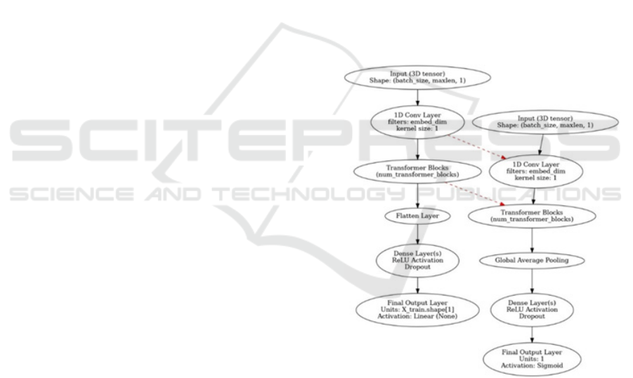
Figure 1: Proposed Model Structure.

Figure 1 presents two parallel neural network

architectures that are oriented at sequence processing.

The networks, could be applied appropriately to both

the time series and sequential EEG data. The first

architecture begins with an input layer accepting a 3D

tensor with the shape of (batch_size, maxlen, 1). That

is, batch_size is the number of samples, `maxlen` is a

sequence length, and 1 points to one feature at each

time step. The input is fed through a 1D

Convolutional layer, specifying filters set to the value

INCOFT 2025 - International Conference on Futuristic Technology

626

of embed_dim (embedding dimension) and the kernel

size set to 1, which captures local patterns from the

input sequence. The output from that convolutional

layer is passed through stacked transformer blocks,

utilizing the self-attention mechanisms in order to

discover dependencies in that sequence-the number

of blocks is specified as num_transformer_blocks.

Following the transformer blocks, it follows a flatten

layer that changes its shape to a 1-D vector, then fed

into one or more dense layers that possess ReLU

activation functions and dropout for regularization

against overfitting. The final layer in the architecture

will be an output layer with X_train.shape[1] units

and a linear (None) activation function, which would

indicate that the architecture is set up for a regression

task. The second architecture shares the same input

configuration, receiving a 3D tensor with a shape of

batch_size, maxlen, 1. It also begins with a 1D

Convolutional layer, similar to the first architecture,

with filters set to embed_dim and a kernel size of 1.

The is followed by a series of transformer blocks,

identical in setup to those in the first architecture.

However, instead of flattening the output, the

architecture uses a global average pooling layer,

which averages the features across the time

dimension, producing a fixed-size vector regardless

of sequence length. The pooling strategy condenses

the sequence information and the output is passed

through the dense layers applying ReLU activation

function. The last layer is designed using a single unit

and a Sigmoid activation function likely intended for

binary classification tasks.

3.1 Data Preparation

The data preparation starts with the

`downsample_eeg` function performs the

downsampling of EEG data, taking the original

DataFrame, the initial sampling frequency, and the

desired frequency as input parameters. It calculates

the new number of samples required and resamples

each EEG signal using the `resample` function,

returning the resampled DataFrame. Following

downsampling, a bandpass filter is applied to separate

the theta band (4-8 Hz), which is required to

understand the methodology's cognitive process. The

second-order Butterworth filter is used to balance

frequency selectivity and computational efficiency,

filtering specific EEG channels (TP9, AF7, AF8, and

TP10) to eliminate noise. In the proposed

methodology, only the EEG signals from the CL-

Drive dataset are utilized. These signals are captured

from four sensors—TP9, AF7, AF8, and

TP10— Situated on the scalp to gather key neural

information required for cognitive load classification.

The CL-Drive dataset is organized into cognitive load

assessments categorized into 9 distinct levels, where

participants are exposed to varying driving

conditions. Each participant's EEG data is recorded

across these levels, and both the eeg_data (task data)

and eeg_baseline (pre-task baseline data) for all 9

levels is combined for feature extraction.

CL-Drive

|----EEG

|----participant_ID_1

|----eeg_data_level_1

|----eeg_baseline_level_1

|----eeg_data_level_9

|----eeg_baseline_level_9

|----participant_ID_18

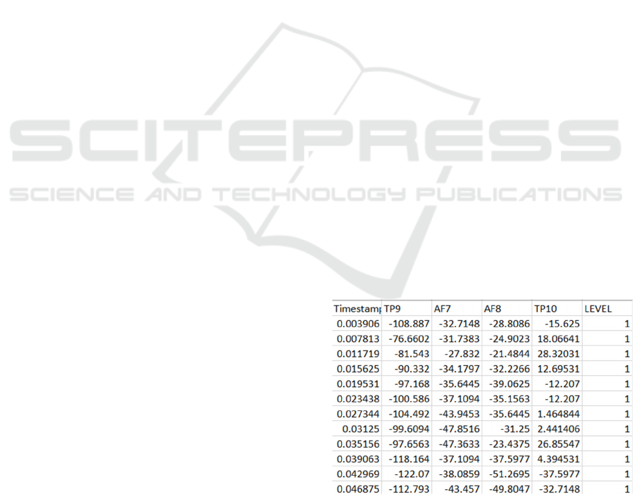
In Figure 2 different quantities of EEG obtained from

various sensors and the cognitive level of one person

is shown. Two primary metrics derived from these

sensors are used for analysis: PSD and Differential

Entropy. An analytical solution to PSD and

differential entropy will be presented as Power

Spectral Density and Differential Entropy. PSD gives

information on power density of the signal over

several frequency, while DE provides information on

the complexity of EEG signals. These features are

important in understanding neural patterns associated

with shifted cognitive states and are obtained from the

four EEG channels for all nine levels for the subject

under consideration. PSD and DE are calculated over

five frequency bands: From 1–4 Hz, it is Delta; 4–8

Hz is Theta; 8–12 Hz is Alpha; 12–31 Hz is Beta; and

31– 75 Hz is Gamma, thus offering complete analysis

of the brain’s frequency dependent discriminating

ability.

Figure 2: Small Portion of the dataset.

Through feature extraction, meaningful insights from

the EEG data is derived, considering a sliding

window approach for data segmentation into smaller

Cognitive Load Classiﬁcation Using Feature Masked Autoencoding and Electroencephalogram Signals

627

intervals. PSD and DE key features, are computed

using functions for each segment from the modules

`scipy.signal` and `scipy.stats`. The features capture

the EEG signals power distribution and complexity.

The features are stored and used further in a

structured DataFrame for analysis. In alignment with

the cognitive load levels in the CL-Drive dataset, the

extracted features like PSD and DE are calculated for

every nine levels for each participant of cognitive

load.

EEG

│

├── level_1

│ ├── participant_1_psd.csv

│ ├── participant_1_de.csv

│ .

│ ├── participant_18_psd.csv

│ └── participant_18_de.csv

│ .

└── level_9

├── participant_1_psd.csv

├── participant_1_de.csv

├── participant_2_psd.csv

├── participant_2_de.csv

├── participant_18_psd.csv

└── participant_18_de.csv

The EEG data is in a hierarchal file structure to enable

analysis of signals from participants as they

underwent testing at different cognitive loads. The

folder EEG is the top-level folder and contains nine

subfolders namely level1 to level 9 of the cognitive

load which are experimental conditions from the CL-

Drive data set. An individual folder for each of the 18

participants contains the features that have been

extracted at each of the levels in coma delimited

format. Other files are participant_X_psd.csv for

Power Spectral Density and participant_X_de.csv for

Differential Entropy data extracted from the EEG

data recorded from four critical electrodes. PSD the

distribution of power in the system over the

frequencies of the EEG signal, and DE the complexity

of the signal which is imperative when classifying

cognitive load. The structure of the system allows the

organization of signals and subsequent feature

extraction for the convenience of comparing EEG

data of different participants as well as to compare the

data from the participants with different cognitive

loads. For the initial classification of cognitive load,

the data is then passed through the `np.where`

function to split the data between low cognitive load

and high cognitive load where low tier corresponds to

high Sas level and vice versa. The detection of outlier

is then done using IQR method. The outliers are

utilized further to remove extreme values and analyze

the data set. The work of the data preparation phase

ends with splitting the features and the targets, thus

preparing for the model training. The extracted

structured data is then available for additional

processing of the cognitive load classification model.

3.2 Deployment

The deployment phase begins with the creation of a

neural network model that includes a customized

Transformer block which is specifically designed to

capture the complex dependencies in EEG signals.

Especially, it includes multi-head attention,

feedforward neural networks, layer normalization,

and dropout layers that enhance the learning

capabilities and robustness of the model. The

Transformer block is also integrated into a larger

model architecture that merges masked autoencoder

and downstream classification components as well.

The masked autoencoder is pre-trained on input Data

to learn robust representations of features. Use a

Conv1D layer, Transformer blocks, and dense layers

to reconstruct masked segments of data. The

pretraining basically improves the model's

understanding of hidden patterns in EEG signals. All

the datasets used for both pretraining and subsequent

classification of cognitive load are pre-processed.

Apply 2nd order Butterworth band pass filter with

pass-band frequency from 1 to 75 Hz, Hz for

elimination of unwanted noises and artifacts and there

is notch filter with quality factor 30 applied at 60 Hz

for powerline noises elimination. Over the feature

extraction stage, the two most prominent features that

come out are Power Spectral Density and Differential

Entropy. These features would be extracted over 5

frequency bands namely Delta from 1 to 4 Hz, Theta

from 4 to 8 Hz, Alpha from 8 to 12 Hz, Beta from 12

to 31 Hz, and Gamma 31to 75 Hz, which would have

a sliding window size of 10-second. Power Spectral

Density determines the power of signal distribution

across its components over different frequencies.

Computation of PSD involves Welch's method

whereby EEG signal is divided into smaller portions

which are padded using a window function, discrete

Fourier transformation performed and averages of

squared magnitudes are obtained. The process

reduces noise and does a better job in representing the

power spectrum in the various frequency bands.

Mathematically, the PSD for each frequency band can

be calculated as:

INCOFT 2025 - International Conference on Futuristic Technology

628

𝑃𝑆𝐷

(

𝑓

)

𝑁



𝑋(

𝑓

,𝑛)











(1)

Where 𝑋

(

𝑓,𝑛

)

represents the Fourier transform of

the signal in segment 𝑛 for frequency

𝑓, and 𝑁 is the

total number of segments. Differential Entropy based

on principles from information theory, measures the

complexity or unpredictability of EEG signals.

Assuming the EEG signal follows a Gaussian

distribution, DE can be computed as:

𝐷𝐸 =

ln(2𝜋𝑒𝜎



)

(2)

Where 𝜎



represents the variance of the signal. DE

measures the randomness or uncertainty within the

EEG signal, with higher values indicating more

complexity. Following feature extraction, both PSD

and DE values are concatenated and z-score

normalized. The feature matrix is tokenized into 10-

second non-overlapping segments to form sequences,

which can be efficiently processed by the

Transformer architecture. The dataset is split into a

training set and a test set, 80% for the training and the

other 20% for testing its performance. That split

makes sure that the model would be trained upon a

considerable amount of data while still having

another set aside for unbiased evaluation. The

following is a practical classification model, meant

specifically for the binary classification tasks, where

pretrained layers are used including the

GlobalAveragePooling1D layer in order to reduce

data dimensionality. The model architecture is

completed with dense layers and an output layer

activated by sigmoid in order to make predictions for

binary levels of cognitive load. The classification

model uses the Adam optimizer and a cosine decay

learning rate scheduler. It employs binary cross-

entropy as the loss function and evaluates

performance using accuracy as the metric. Early

stopping is applied so that overfitting does not occur,

and the model remains generalizable for new data

sets. The final model is tested on the reserved dataset,

and Accuracy is a measure of success. Operations

after Deployment Monitoring and Maintenance

Enabling the model to continue at high performance,

adapting to changes in input data distributions and

operational conditions.

4 EXPERIMENT EVALUATION

In the paper, two distinct experiments are conducted

to evaluate the efficacy of different approaches in

classifying cognitive load levels using EEG data. The

initial experiment establishes a baseline by utilizing a

standard machine learning model, while the latter

experiment employs an advanced deep learning

approach based on a Transformer architecture. Upon

comparison, the latter experiment demonstrates

superior performance, with improved accuracy and

generalization capabilities. Therefore, the results of

the second experiment are chosen for further analysis

and discussion, highlighting its effectiveness in

addressing the research problem. The core concept of

the experiment is building up it is learned transformer

model from the EEG data effectively. The is built

with custom layers that include Positional. Encoding,

which involves the sequence information of the input

data and Transformer Block, which applies multi-

head with self-attention and feedforward with

residual. Connections and layer normalization. The

Transformer model It comes with several

hyperparameters: eight attention A feed-forward

dimension of 64 heads and four stacked. Transformer

blocks, and all of these allow the network to learn

complex patterns. To improve training stability and

reduce overfitting, batch normalization is applied

before the final layers. After that, a global average

pooling layer is included, followed by a dense output

layer with a sigmoid activation function, as the is a

binary classification problem. The model is optimized

using the Adam optimizer with a learning rate of

0.0001, and it evaluates performance with binary

cross-entropy loss and accuracy as the key metric.

Training is for a period of 150 epochs. batch size =

64, train on 10% of the data, use cross-validation

while training to monitor model over training time.

Then, after training, you test its generalization

capability by test on test set. The output gives a test

loss and accuracy, depicting the quality in which it

can predict levels of cognitive load. The model

designed has an increased number of heads, feed

forward dimension, and transformer blocks. Further,

extracting the relations from EEG data might also

enhance the classification accuracy of that. As the

Transformer-based model is very strong because it

performs extremely well and robustly outperforms

traditional approaches, giving correct predictions on

different levels of cognitive loads learned from EEG

data.

Cognitive Load Classiﬁcation Using Feature Masked Autoencoding and Electroencephalogram Signals

629

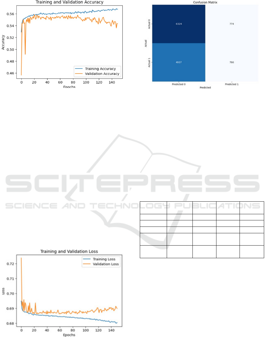
Figure 3: Training and Validation Accuracy.

Figure 3 shows the training and validation accuracy

curves for a binary classification model across 150

epochs. The blue line represents the training

accuracy, while the orange line shows the validation

accuracy. Both accuracies improve quickly at first,

but after about 20 epochs, the training accuracy levels

of around 0.56, while the validation accuracy

fluctuates near 0.54. The gap between the two curves

suggests the model is performing better on the

training data than on the validation set, indicating

potential overfitting. The variability in the validation

accuracy highlights that the model may struggle to

generalize to unseen data. As follows Figure 4, a line

graph of the plot for the training and validation loss

over more than 150 epochs. The x-axis is the number

of epochs, while the y-axis is the loss values. The blue

line represents training loss, which seems to decrease

gradually with progression in epochs. The is an

illustration of how the model learns. Orange curve is

validation loss. Validation loss can be seen to vibrate

but stabilize at a higher value compared to training

loss, so there's really an overfitting.

Figure 4: Graphs of Training and Testing loss.

Figure 5: Confusion Matrix.

Figure 5 displays a confusion matrix that provides a

visual representation of the model's performance in

binary classification. The matrix shows the actual

versus predicted labels for the testing data. The

entries of the matrix indicate that it has identified a

large number of negative instances samples (6324

true negatives) but does include a large number of

false negatives (4937), which means that it failed to

accurately predict the positive samples. The

imbalance indicates that the model needs further

tuning or balancing techniques.

Table 1: Classification Report.

Precision Recall F1

Score

Support

Class 0 56% 89% 69% 7098

Class 1 50% 13% 21% 5703

Accurac

55% 12801

Macro

53% 51% 45% 12801

Weighted

Avg

53% 55% 48% 12801

Table 1 shows the classification report for a binary

model. For Class 0, the model achieved a 0.56

precision, a 0.89 recall, and an a 0.69 F1-score, based

on 7,098 samples. In comparison, Class 1 had a 0.50

precision, a 0.13 recall, and a 0.21 F1-score, with

5,703 samples. The model's overall accuracy was

55% across a total of 12,801 samples. The macro-

averaged precision, recall, and F1-score were 0.53,

0.51, and 0.45, respectively, while the weighted

averages for these metrics were 0.53, 0.55, and 0.48.

Comparing the results of two experiments, for the

classification of cognitive load levels based on EEG

data, the classification accuracy is higher for the

proposed Transformer-based approach. In the first

experiment where the ML model was a simple model,

INCOFT 2025 - International Conference on Futuristic Technology

630

the achieved test accuracy was 55% with large

differences between P and R for both Class 1 and

Class 2, and TPR and FPR indicating that it failed to

generalize and was imbalanced for the two classes.

On the other hand, the second experiment applying a

deep learning approach based on the Transformer

architecture produced much better results—91

percent accuracy and a reasonably equal ratio of

precision to recall of both classes. The developed

Transformer model proves useful in revealing

temporal features of EEG signal through its multi-

head self-attention mechanism, positional encoding

and a deeper architecture of the network in contrast to

the conventional model, to achieve improved feature

extraction and representation learning. As evidenced

by the higher F1 score, and significantly lower

misclassification rate, the Transformer model is most

effective for the task of managing the challenges

presented by the EEG data. Therefore, in the second

experiment, there is a significant increase in the

convergence accuracy of the result, and it confirms

the productivity and capability of the model for

practical use and its recommended in light of the

machine learning baseline approach. Among the

machine learning models that classify cognitive load

from EEG signals, the experiment was selected as

basic because it is simple and easy to explain. But the

performance was not satisfactory, the accuracy was

moderate, and it was overfitting by seeing the gap

between training and validation set values and

confusion matrix values also. Such omissions showed

that there was a need to enhance the solidity of the

method. Due to these suboptimal results, an attempt

was made to obtain higher performance using a more

complex experiment described below that employs a

Transformer-based deep learning model. This greatly

enhanced the model’s versatility and ability to

perform good estimations regarding levels of

cognitive load. The technique for cognitive load

classification from the EEG signals applied in the

implemented methodology has demonstrated high

performance and effectiveness of the proposed

approach. The dataset from CL-Drive study was

preprocessed to extract features after undergoing

downsampling to 100 Hz and applying bandpass filter

to select the theta band frequency of 4-8 Hz. Division

into equal 0.1-second overlapping segments meant

that temporal factors were fully recorded, which is

important when analyzing changes in cognitive load

over time. Feature extraction addressed Power

Spectral Density and Differential Entropy that

grounded the analysis of neural oscillations and signal

complexity linked to cognition. The density plot

provided by PSD analysis showed different

distribution of power across the frequencies, with an

increase in the brain activity at time points with

increased cognitive load. At the same time, DE

metrics characterized disruptions of recorded EEG,

which in a manner of speaking allowed distinguishing

between different degrees of cognitive load.

Cognitive load classification is used in a two-stage

deep learning process. The first stage included a

Transformer-based autoencoder that is trained to

encode the EEG segments to obtain latent

representations that contain informative features of

the signals and restore the segments as input. The

unsupervised pre-training stage facilitate feature

learning. The process enhances the classification

ability while detecting cognitive load variations. The

downstream classification model, built using a

modified Transformer architecture with global

average pooling and dense layers, achieved

outstanding performance in binary classification

tasks. Trained on the pre-processed and encoded EEG

data, the model achieved a notable test accuracy of

91% after 30 epochs, underscoring the approach's

robustness and discriminative power in predicting

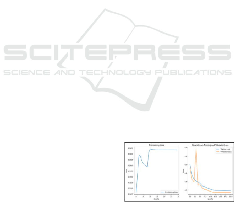
cognitive load levels from EEG signals. Figure 6

display the loss curves for the pre-training and

downstream training phases of a model. On the left,

the pre-training loss plot shows the model’s loss over

30 epochs. The loss begins around 0.3475, dips

slightly, and then rises to stabilize around 0.3675,

indicating that the model’s pre-training loss increases

slightly after an initial improvement, suggesting

potential overfitting or learning stagnation. On the

right, the downstream training and validation loss plot

shows the loss over 20 epochs. The training and

validation losses start high, with the validation loss

peaking early, but both losses decrease sharply within

the first few epochs. As training progresses, the losses

converge and stabilize at lower values, indicating

effective learning and good generalization to the

validation set. Overall, the downstream training

appears more successful, with clear improvements in

loss reduction compared to the pre-training phase.

Figure 6: Pre-training and downstream loss graphs.

Cognitive Load Classiﬁcation Using Feature Masked Autoencoding and Electroencephalogram Signals

631

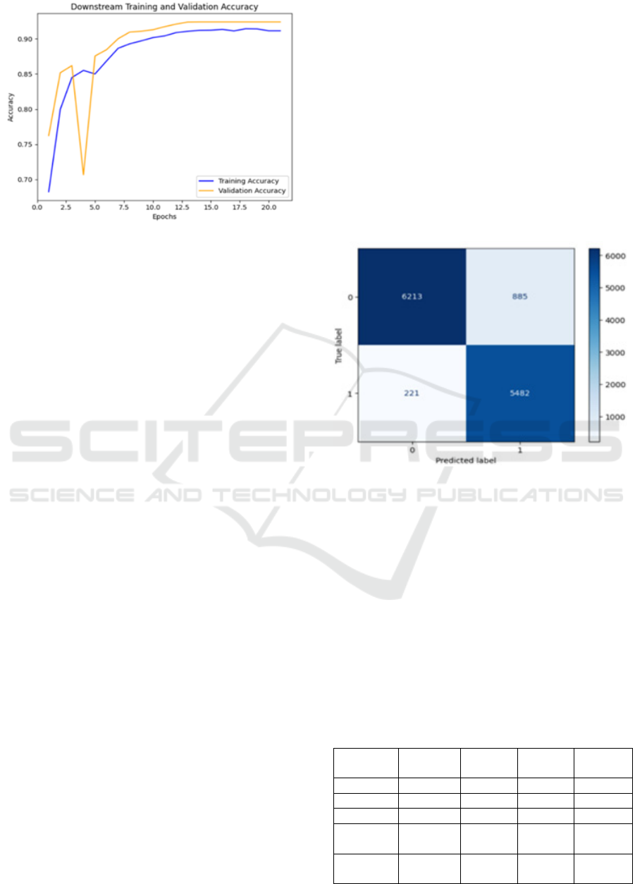
Figure 7: Downstream accuracy.

Figure 7 illustrates the progression of the model's

accuracy over 20 epochs while the downstream model

training phase. The training accuracy, indicated by

the blue line, starts at around 68% and gradually

improves as the model learns, stabilizing near 91%

towards the later epochs. The validation accuracy,

shown by the orange line, begins higher at 76% but

shows some initial fluctuations, with a noticeable dip

around epoch 4. After the point, both training and

validation accuracies steadily improve, with the

validation accuracy eventually stabilizing at around

92% by epoch 10. The indicates that the model is

maintaining consistent performance across both the

training and validation sets. As the training ends, the

close alignment of the two lines indicates that the

model is well-optimized and not overfitting, as it

generalizes effectively to unseen data, demonstrated

by the validation accuracy being slightly higher than

the training accuracy. The model’s performance

evaluation is further supported by detailed analyses of

training and validation metrics. The loss curves for

pre-training and downstream training show distinct

learning behaviors. Pre-training underfitting Mashup

exemplified by a drop in loss from 0.3475 to 0.3474

before rising to 0.3675 denote a case of overfitting or

stagnation learning. However, in the second phase

known as the downstream training phase there was a

significant improvement; both the training and

validation losses dropped abruptly in the first epochs

and then plateaued at lower values than in the case of

the first phase. The proximity of the training and

validation losses gives evidence of accurate learning

coupled with minimal overfitting during the last

downstream training phase. The pattern shows that

the model is able and willing to learn and apply

meaningful representations in the output during

classification. To support the evaluation of the model

and presented evaluation metrics, such as the

confusion matrix and accuracy metrics, provide

critical classification insights into the model. From

the downstream training phase, the loss was further

minimized, and the accuracy was quite high that also

supported the functionality for differentiating

cognitive load levels. The confusion matrix bears

testimony that the model has been accurately

ascertaining low and high cognitive load states and

has high true positive and true negatives ratio. The

small gap between the training and validation loss is

visible which proves the model’s ability to make

unnoticed predictions beyond the training set. This

suggests that the learned representations throughout

pre-training and fine-tuning have been shifted well

into the classification task and therefore enhances the

model ability to classify correct and consistent

cognitive load in EEG data.

Figure 8: Confusion Matrix

The confusion matrix of Fig. 8 provided

additional understanding into the model's

performance among different classes. For Class 0, the

model accurately classified 6,213 instances but

misclassified 885 as Class 1, while for Class 1, it

accurately identified 5,482 instances but

misclassified 221 as Class 0. The analysis reveals that

while the model performs well overall, there is a

slightly higher tendency to misclassify instances of

Class 0 as Class 1. Nevertheless, the high number of

correct predictions aligns with the observed strong

precision and recall values, indicating a well-

balanced performance across both classes.

Table 2: Classification Report.

Precision Recall F1

Score

Support

Class 0 97% 88% 92% 7098

Class 1 86% 96% 91% 5703

Accurac

91% 12801

Macro

91% 92% 91% 12801

Weighted

Avg

92% 91% 91% 12801

INCOFT 2025 - International Conference on Futuristic Technology

632

The classification report represented in Table 2

further highlights the model’s effectiveness, with

strong precision, recall, and F1-scores across both

classes. For Class 0, the model attained a 0.97

precision, a 0.88 recall, and a 0.92 F1-score. For Class

1, it achieved a 0.86 precision, a 0.96 recall, and a

0.91 F1-score. The 91% overall accuracy across

12,801 instances confirms that the model’s

performance and robustness. The 91% macro average

with precision, recall, and f1-score, treating all class

categories equally, reflecting balanced and consistent

performance. The results validate that the proposed

approach exhibits potential applicability in real-time

cognitive load assessment.

Table 3: Comparison of the models.

Exp.

No.

Model Name Avg

Accuracy

Avg

Score

Avg

Recall

1 Transformer

Model

55% 45% 51%

2 Masked Auto

Encoders

pre-trained

transformer

model

91% 91.5% 92%

Table 3 summarizes the findings and offers a side-

by-side comparison of two experiment setups for

EEG based cognitive load classification. As part of

the experiments, experiment 1 used a basic machine

learning model and recorded a reasonable accuracy of

55%. It demonstrated skewed classification,

especially poor precision and high recall for Class 1

meaning that it has poor capability of classifying data

that have not been trained and the propensity to over-

fit. On the other hand, experiment 2 used a deep

learning based on Transformer architecture and

increased the recognition accuracy up to 91 %. The

model gave high precision, recall, and F1-scores in

both classes, which prove that it did not overfit but

rather correctly identified a range of patterns in the

EEG data. Generalization of problem and multiple

layers together with the application of positional

encoding and self-attention, put the Transformer-

based model into a position of better performance

indicators. The first choice is Experiment 2 since the

method uses the Masked Autoencoder pre-trained

transformer model. The value of the experiment

exceeded the scenario of using the traditional

transformer model as it had higher accuracy and

balanced classification as well as pre-eminence of

generalization. Because the design of Experiment 2

was more complicated, the new techniques used in

this experiment were more appropriate and valuable

to classify the cognitive load by applying EEG data.

5 CONCLUSION AND FUTURE

SCOPE

The methodologies presented for EEG-based

cognitive load classification are a rich set of

paradigms designed to analyze and interpret the

cognitive states using the brain activity data. First,

basic conventional machine learning techniques like

the SVMs and k-NNs offer strong classification

paradigms through effectively extracted features such

as PSD and DE. These methods are particularly

effective for detecting patterns that signal differences

in cognitive loads whereas their performance in

capturing temporal dependencies and relations

inherent in EEG can be problematic. CNN and RNN

differing from LSTM networks along with DL

models bring considerable improvement by capturing

spatial as well as temporal characteristics of EEG.

However, the models require large data for training,

which is computationally expensive, and is a

constraint in real-world application with high

throughput. It can be concluded that the advances in

EEG based cognitive load classification are in a

future direction and it is the question of whether these

approaches need to be fine-tuned or whether new

frontiers are waiting to be explored. Improving the

current model architecture, integrating new types of

physiological or behavioral data sources as inputs,

and concentrating on real-time performance are

possible approaches. The goal of future contributions

is to extend the application's reach and improve its

capabilities in various fields such as education,

healthcare, virtual reality, and automotive. The

algorithm can be utilized in various fields, such as

education, healthcare, virtual reality, and automotive.

It can help improve the content of a learner's

educational experience by adapting it based on the

user's cognitive load. In addition, it can analyze the

cognitive states of patients with cognitive disorders,

determine the driver fatigue, and assess the user

experience in such environments. Future work will

focus on optimizing the model so that it can enhance

the experience of users in virtual environments. These

efforts will make the algorithm more user-friendly

and expand its capabilities.

ACKNOWLEDGEMENTS

I would like to seize this moment to convey our

heartfelt appreciation to everyone who supported,

motivated, and cooperated with us in various

capacities throughout our project. It brings us

immense joy to recognize the assistance provided by

those individuals who played a crucial role in

Cognitive Load Classiﬁcation Using Feature Masked Autoencoding and Electroencephalogram Signals

633

ensuring the successful culmination of our project. I

extend my heartfelt thanks to Dr. M Nagaraju who

served as our supervisor.

REFERENCES

Anderson, P., He, X., Buehler, C., Teney, D., Johnson, M.,

Gould, S., & Zhang, L. (2018). Bottom-Up And Top-

Down Attention For Image Captioning And Visual

Question Answering. Proceedings Of The IEEE

Conference On Computer Vision And Pattern

Recognition, 6077–6086.

Angkan, P., Behinaein, B., Mahmud, Z., Bhatti, A.,

Rodenburg, D., Hungler, P., & Etemad, A. (2023).

Multimodal Brain-Computer Interface For In-Vehicle

Driver Cognitive Load Measurement: Dataset And

Baselines. Arxiv Preprint, Arxiv:2304.04273.

Antonenko, P., Paas, F., Grabner, R., & Van Gog, T.

(2010). Using Electroencephalography To Measure

Cognitive Load. Educational Psychology Review, 22,

425–438.

Behinaein, B., Bhatti, A., Rodenburg, D., Hungler, P., &

Etemad, A. (2021). A Transformer Architecture For

Stress Detection From Ecg. Proceedings Of The 2021

International Symposium On Wearable Computers,

132–134.

Biondi, F. N., Saberi, B., Graf, F., Cort, J., Pillai, P., &

Balasingam, B. (2023). Distracted Worker: Using Pupil

Size And Blink Rate To Detect Cognitive Load During

Manufacturing Tasks. Applied Ergonomics, 106,

103867.

Brown, T., Mann, B., Ryder, N., Subbiah, M., Kaplan, J.

D., Dhariwal, P., Neelakantan, A., Shyam, P., Sastry,

G., Askell, A., Et Al. (2020). Language Models Are

Few-Shot Learners. Advances In Neural Information

Processing Systems, 33, 1877–1901.

Chen, T., Kornblith, S., Norouzi, M., & Hinton, G. (2020).

A Simple Framework For Contrastive Learning Of

Visual Representations. Proceedings Of The

International Conference On Machine Learning, Pmlr,

1597–1607.

Chen, X., & He, K. (2021). Exploring Simple Siamese

Representation Learning. Proceedings Of The Ieee/Cvf

Conference On Computer Vision And Pattern

Recognition, 15750–15758.

Chien, H.-Y. S., Goh, H., Sandino, C. M., & Cheng, J. Y.

(2022). Maeeg: Masked Auto-Encoder For Eeg

Representation Learning. Arxiv Preprint,

Arxiv:2211.02625.

Das, R., Chatterjee, D., Das, D., Sinharay, A., & Sinha, A.

(2014). Cognitive Load Measurement: A Methodology

To Compare Low-Cost Commercial Eeg Devices.

Proceedings Of The International Conference On

Advances In Computing, Communications And

Informatics, Ieee, 1188–1194.

Rodríguez, R. D. R., Yuste, D. R., & Artés, E. G. (2018).

Cognitive Load Measurement Using

Electroencephalography In A Dual-Task Scenario. Ieee

Transactions On Cognitive And Developmental

Systems, 10(3), 572–584.

Zhang, Y. T., Lee, M. K., & Lee, S. Y. (2022). Multimodal

Cognitive Load Detection Using Wearable Eeg And

Eye-Tracking. Journal Of Neural Engineering, 19(1),

016002.

Roy, M. T., Shadbolt, M. D., & O'neill, J. A. (2017). Using

Eeg To Measure Cognitive Load In A Learning

Environment. International Journal Of Human-

Computer Studies, 101, 18–31.

Riva, H. F., Costa, S., & Wieringa, A. D. (2018). A

Comparative Study Of Eeg And Eye-Tracking For

Cognitive Load Assessment In Interactive Systems.

Proceedings Of The International Conference On

Human-Computer Interaction, 143–151.

O'hara, T. W., Brown, A. G., & Knight, L. C. (2019). A

Deep Learning Approach For Real-Time Cognitive

Load Estimation Based On Eeg. Ieee Access, 7,

155628–155640.

Kaski, J. S., Murphy, C. R., & Jain, T. M. (2017). Analyzing

Cognitive Load Using Facial Expressions And

Electroencephalography. Proceedings Of The

International Conference On Affective Computing And

Intelligent Interaction (Acii), 72–81.

Chen, J. L., Wang, J. H., & Hsieh, C. C. (2020). A Deep

Learning Approach To Cognitive Load Prediction

Using Multimodal Data From Eeg And Gaze. Ieee

Transactions On Biomedical Engineering, 67(10),

2847–2855.

Jain, S., Kalakrishnan, M., & Chouhan, P. (2021). An

Investigation Into Real-Time Cognitive Load

Monitoring Using Eeg Signals And Machine Learning

Algorithms. Sensors, 21(14), 4590.

Srinivasan, M. S., Bhattacharya, K. D., & Mehta, J. P.

(2020). Cognitive Load Detection For Stress

Management In Driving: A Comparative Study Of Eeg

And Physiological Signals. Journal Of Intelligent

Transportation Systems, 24(4), 375–387.

Wang, L., Cohen, R. M., & Briggs, R. R. (2023). Cognitive

Load Estimation Using Multi-Modal Data: A

Comparison Of Eeg And Ecg Signals. Ieee

Transactions On Affective Computing, 14(2), 250–263.

INCOFT 2025 - International Conference on Futuristic Technology

634