IDAT: An Interactive Data Exploration Tool

Nir Regev, Asaf Shabtai and Lior Rokach

Dept. of Software and Information Systems Engineering, Ben-Gurion University of the Negev, Beer Sheva, Israel

Keywords: EDA (Exploratory Data Analysis), Neural Network, SQL, Supervised Learning.

Abstract: In the current landscape of data analytics, data scientists predominantly utilize in-memory processing tools

such as Python’s pandas or big data frameworks like Spark to conduct exploratory data analysis (EDA). These

methods, while powerful, often entail substantial trade-offs, including significant consumption of time,

memory, and storage, alongside elevated data scanning costs. Considering these limitations, we developed

iDAT, a cost-effective interactive data exploration method. Our method uses a deep neural network (NN) to

learn the relationship between queries and their results to provide a rapid inference layer for the prediction of

query results. To validate the method, we let 20 data scientists run EDA (exploratory data analysis) queries

using the system underlying this method. We show that it reduces the need to scan data during inference

(query calculation). We evaluated this method using 12 datasets and compared it to the latest query

approximation engines (VerdictDB, BlinkDB) in terms of query latency, model weight, and accuracy. Our

results indicate that the iDat predicted query results with a WMAPE (weighted mean absolute percentage

error) ranging from approximately 1% to 4%, which, for most of our datasets, was better than the results of

the compared benchmarks.

1 INTRODUCTION

The emergence of big data offers the potential to gain

unprecedented insights, yet this comes with the

challenge of increased processing latency and greater

demand for computational resources when querying

extensive datasets (Chaudhuri et al., 2017).

Frequently, data scientists engaged in exploratory

data analysis must handle large datasets, repeatedly

querying them to statistically describe and extract

insights and relationships.

These tasks require a query engine that is rapid,

efficient, and cost-effective but does not depend on

delivering precise results. For such tasks, providing

approximate estimations of the characteristics and

statistics of the data is often adequate. In these

instances, the use of Approximate Query Processing

(AQP) methods becomes particularly advantageous.

There are other scenarios where a data estimate is

enough, such as reporting, visualization, fast decision

making, and even process simulation. Moreover,

several factors must be considered when evaluating

the applications of query approximation: (1) raw data

may not always be accessible, occasionally due to

privacy restrictions or compliance with GDPR

regulations; (2) maintaining and processing raw data

in a database can be expensive; and (3) raw datasets

may exhibit inconsistencies or have missing data.

Ultimately, when data volumes exceed the

capacity of a single machine, data processing platform

providers such as Hadoop, Spark, and Google Cloud

Dataflow tackle this challenge by scaling out

resources. This strategy, while addressing volume

issues, can become inefficient and cost-prohibitive for

managing large and distributed data sources

(Sivarajah et al., 2017). In addition, this approach

encounters difficulties when there is a need for real-

time data interaction and a high degree of

responsiveness from users or systems. Consequently,

research indicates that data exploration can be

conducted effectively using approximate methods

(Slezak et al., 2018).

That said, the concept of AQP is robust and

possesses disruptive market potential. Thus, the

ability to answer analytic queries "approximately," at

a fraction of the cost required for traditional query

execution, is particularly appealing. Leveraging the

capabilities of AQP could significantly enhance our

ability to quickly and efficiently explore large

volumes of data (Li and Li, 2018).

This forms the basis of our motivation to develop

a swift EDA tool in for data scientist and analysts. To

Regev, N., Shabtai, A., Rokach and L.

IDAT: An Interactive Data Exploration Tool.

DOI: 10.5220/0013597800003967

In Proceedings of the 14th International Conference on Data Science, Technology and Applications (DATA 2025), pages 603-613

ISBN: 978-989-758-758-0; ISSN: 2184-285X

603

firmly back up this motivation, let us take a

hypothetical use case where a group of 10 analysts

explore the relationship between life expectancy and

socioeconomic factors (such as income). A cloud

storage with 20 data attributes is available for this task

and populates the related data for every adult in the

world (5.3 billion adults globally) and takes

approximately 5.3 TB (20 fields×50 bytes= 1KB per

adult). To calculate the required number of queries for

such research, we will assume that only three

continuous variables are taken into the analysis: (1)

income, (2) expenditure (spending on goods and

services) and debt (loans and mortgages) where each

factor is binned into 10 levels. The total combinations

of these factors will increase to 1000, which is

approximately the number of queries required for a

single analyst to execute. If every analyst explores

different sets of factors, we can assume that

approximately 10,000 queries will be needed to

calculate the average life expectancy grouped by each

city (10,000 cities worldwide) for this research, with

each scanning 5.3 TB of data. For simplicity, we

assume that there is no storage cost, and only the

compute cost will be considered. This will incur a

compute cost of 83$ for a single query (based on

AWS Lambda: 0.00001667$ per GB processed).

Overall costs for all queries are 830,000$. Scanning

5TB is estimated to take 11.5 hours (based on a high-

speed connection of 1 Gb per second).

In summary, the described use case takes

significant resources in terms of costs and time to

perform data exploration tasks for such research.

Naturally, the above pipeline is not feasible for most

companies; this is the reason why analysts will sample

a fraction of the data and risk introducing sampling

biases that can skew research results. The method we

developed for this applied research is based on this

work (Regev et al., 2021) and may serve as a good fit

to the described use case. We significantly improved

the work of (Regev et al., 2021) by enriching the

query structure to support complex SQL logic such as

Join/Outer Join operations, added statistical functions

(i.e. median, 25%, 75%) and most importantly added

support to scenarios where raw dataset changes

quickly. In addition, contrary to (Regev et al., 2021),

we tested iDat in real EDA scenarios letting data

scientists and analysts interact with it. The AQP

approach may introduce slight inaccuracies, and the

trade-off is acceptable for use cases where cost, speed,

and efficiency are prioritized over exact precision. In

this research, we specifically focus on data

exploration which is a common task for data scientist

and analysts. Data exploration in large datasets can be

resource intensive and requires significant

computational power to query, aggregate, and

visualize vast amounts of data. This process may

incur high costs in terms of processing time, cloud

storage, and compute resources, especially when

repeated queries or full dataset scans are involved. In

addition, slow query performance can hinder analyst

productivity, delaying insights and decision making.

These summaries the justification for a light ML

(Machine Learning) based SQL query executor.

Previous methods for query approximation were

predominantly concentrated on constructing

representative data samples. The efficacy of these

approaches depends on the use of statistical methods

to furnish a confidence interval for the approximated

results. However, for complex and dynamic datasets,

innovative sampling methods must be employed and

recalculated frequently to ensure that they remain in

sync with the database (Mozafari and Niu, 2015). In

addition, other techniques have utilized data

summaries, prepared in advance, to represent raw data

in compact and aggregated form (Cormode et al.,

2012). Finally, existing solutions based on this

approach aim to approximate predefined query

configurations (Cuzzocrea and Saccà, 2013), like the

design of online analytical processing (OLAP) cubes.

This raises concerns about the applicability of these

solutions for the exploration of generic data (Nguyen

and Nguyen, 2005). Other proposed methods focus on

facilitating query approximation in streaming and

interactive systems through the use of distributed data

processing engines such as Hive, Spark SQL, Impala,

Amazon Redshift, and Presto (Ramnarayan et al.,

2016), (Agarwal and Mozafari, 2013).Although these

methods can provide accurate and rapid results,

depending on the size and tuning of the Spark

cluster—they can be cost prohibitive and require the

ability to store and access the data.

In this paper, we present an iDat - a method based

on a NN to provide a rapid interactive EDA tool. The

primary motivation behind this research is to reduce

query latency, reduce computational expenses, and

maintain high accuracy in model predictions. We

show that our selected approach significantly reduces

data scans and query latency, particularly for large-

scale datasets. Consequently, it is suitable for use in

exploratory analysis and real-time dashboards at cost-

sensitive environments. Our method consists of these

phases: First, a set of analytical queries is generated

(without prior knowledge required on the raw

dataset). In the second phase, we utilize an embedding

method to represent the queries in numeric format.

Last, we train deep sequential NN (RNN) model is

trained to learn approximations for query results,

based on the training set.

DATA 2025 - 14th International Conference on Data Science, Technology and Applications

604

We tested this method in the field by allowing 20

data scientists and analysts to execute data

exploration queries using our method. iDat was

evaluated on 12 datasets from the technology industry

and evaluated the accuracy of the model by

comparing the model predictions for queries (driven

by data scientists and analysts) with the true labels

acquired from the database. We also measured query

latency derived from the model inference time. The

results show that our method predicted the results of

the query with a normalized root mean squared error

(WMAPE) ranging from approximately 1 to 4 %. In

terms of execution latency, the mean query latency

(mean QL) ranges from approximately 2 ms/q

(milliseconds per query) to 32 ms/q. We also

evaluated our method’s performance on large batches

of queries (processed in parallel on a GPU).

In summary, the contributions of this paper are as

follows:

• we introduce a novel method for producing a

lightweight sequential NN which provides a

high query throughput.

• we propose an effective query processing

method for practical data exploration use-cases,

with extremely fast query response times for big

data platforms.

• Finally, we make our code and datasets publicly

available.

@https://anonymous.4open.science/r/aqp\_jurassic-

5B0E

2 RELATED WORK

In the following sections, we address 4 current

methods with which interactive data exploration may

be carried out: (1) real-time processing, (2) ML based

method, (3) In-memory processing, and (4)

processing through data summaries.

Real-time processing. Introduced in 2015, the

SnappyData engine (Ramnarayan et al., 2016) was

specifically engineered to facilitate query

approximation within streaming and interactive

systems. This foundational work featured in the initial

SnappyData publication was based on the knowledge

derived from the BlinkDB project (Agarwal and

Mozafari, 2013). Additionally, Spark, an in-memory

data processing engine distributed across systems, is

designed to optimize smart query caching (termed as

delta update queries) and employs confidence

intervals to mitigate data loss. Spark further enhances

performance by managing on-line aggregation, which

entails processing a small segment of the entire

dataset. This approach enables immediate

presentation of the approximated preliminary results

(Zeng et al., 2015).

ML method for data processing. The database

research community has developed innovative ML-

based techniques for Approximate Query Processing

(AQP) that substantially accelerate the provision of

approximate query results, achieving speeds orders of

magnitude faster than traditional DBMS methods

used for calculating exact results. In these papers

(Thirumuruganathan et al., 2013), (Savva et al.,

2020), researchers used deep generative models,

particularly variational autoencoders (VAEs), to

execute aggregate queries in interactive applications

such as data exploration and visualization. This

research (Savva et al., 2020) also incorporated

machine learning models to approximate the

aggregated SQL queries. Models such as gradient

boost machines (GBMs), XGBoost, and LightGBM

were trained to predict the results of aggregated

queries. The efficacy of our method relative to

established methods is summarized in Table 1.

In-memory data processing with sampling. In

contexts where the volume of data is extensive and

memory capacity is constrained; sampling can

facilitate in-memory processing. Various

methodologies have been developed to approximate

database queries, predominantly through the

execution of queries on intelligently selected data

samples (Mozafari and Niu, 2015). These techniques

employ statistical methods to provide an estimated

result within a specified confidence interval.

Although numerous studies have examined the

advantages of data sampling (Bagchi et al., 2007),

(Babcock et al., 2001), (Chuang et al., 2009), their

integration into streaming engines remains limited

(Chandramouli et al., 2014), (Zaharia et al., 2013). An

exception is the SnappyData project (Ramnarayan et

al., 2016), an analytics database optimized for

memory usage that uses the High-Level Accuracy

Contract (HAC), a concept which was implemented

in VerdictDB (Mozafari et al., 2018). VerdictDB

operates at the driver level, intercepting analytical

queries issued to the database and rewriting them into

another query that yields sufficient information to

compute an approximate answer. The predominant

approach in Approximate Query Processing (AQP)

systems involves the use of stratified sampling, which

relies on prior knowledge of data distributions,

although such knowledge is not always available (Li

an Li, 2018), (He et al., 2018), (Savva et al., 2020).

However, such methods that use uniform random

sampling are less effective for "Group By" queries,

which is crucial in conducting exploratory data

analysis. In contrast, stratified sampling has been

IDAT: An Interactive Data Exploration Tool

605

shown to be more efficient for such tasks (Acharya et

al., 1999). However, stratified sampling methods

generally require significant pre-processing time for

data preparation to approximate a known set of

queries. Although this approach may be effective for

certain applications, it can be inefficient for

interactive data exploration, which typically involves

ad hoc and unforeseen queries (Galakatos et al.,

2017), (Acharya et al., 1999).

Processing with data summaries. With this

approach, AQP is applied to data summaries that were

prepared in advance (Cormode et al., 2012). This

approach, along with the sampling methods discussed

above, is considered complementary (Ramnarayan et

al., 2016). Existing mechanisms for constructing data

summaries are tailored to approximate predefined

query configurations (Cuzzocrea and Saccà, 2013),

analogously to the way that OLAP cubes are designed

to compute predetermined data aggregations.

These strategies evoke concerns about their

suitability for generic data exploration, which

requires a broad spectrum of queries to effectively

summarize the data (Nguyen and Nguyen, 2005).

Such queries might not always be available or

predefined. The concept of employing data

summaries to reduce query latency was initially

proposed by (Jagadish et al., 1998), who used

histograms to this end. Furthermore, there exists a

substantial body of research dedicated to the

implementation of data summaries in relational

database management systems (DBMSs) (Gibbons et

al., 1997).

3 PROPOSED METHOD

Our method utilizes a ML supervised learning

pipeline starting by building a training set of SQL

queries, encoding the queries, labelling the queries

and finally fitting a deep sequential NN (Neural

Network in RNN architecture). The final model (NN)

is used to predict new user SQL queries without

scanning the raw data set. First, we define the query

structure and the terminology of the data scheme. As

an example, assume a table ‘life_exp’ that includes

data on health status, as well as many other related

factors for all countries. The table includes the

following columns: ‘country’, ’city’, ’income’,

’gender’, year’, ’status’, ’Life Expectancy’, ’Adult

mortality’, ’expenditure’ and more. The method is

designed to generate many queries that conform to a

query template defined by the following:

1) S =< s1,s2, ...si > – denotes the set of optional

aggregation functions (e.g. avg, count).

2) col(n) – denotes a numeric data column in the

dataset (e.g., ‘income’).

3) col(d) – denotes a discrete (categorical) data

column in the data set (e.g. ‘city’ ‘gender’).

4) a

(col) – denotes an aggregation function ai ∈ A

that is applied on valid col col (either col(n) or

col(d)) in a ’SELECT’ query clause (e.g.,

avg(‘Life expectancy’), max(‘Life expectancy’),

or count()).

range

col

(

(f,c) – a ‘range’ constraint argument

defined on a numeric data column col(n), where

f is a floor edge (low) in the range and c is a

ceiling edge (high) in the range through the

values of col(n). The ‘range’ constraint is

executed as a ‘between’ SQL operator.

exist

col

(

) – an ‘exist’ constraint argument

defined on a discrete data column col(d), where

(mi) is a valid list of values from col(d) such that

all records associated with any value from this

list will return in the results set.

3.1 Analytical Queries Structure

iDat supports queries with multiple ai(col) grouped by

multiple col(d) columns. Although this enables

flexibility in exploring and analysing large datasets, it

poses the following two challenges: (1) Different

ai(col) (aggregated columns) may distribute very

differently, and (2) the challenge of predicting an

output which may have varying dimensions. The

latter stems from the fact that a "Group By" query can

return a table of one or more rows, as shown by the

example in Table II, which presents the result of the

following example query:

SELECT city, gender, avg(’Life expectancy’)

FROM life_exp le RIGHT OUTER JOIN geo_country

gc ON le.city = gc.c_code WHERE income between

(10000 and 20000) AND expen-diture between (50000

and 60000) GROUP BY city, gender

To tackle these challenges, we represent each

"Group By" query into multiple ‘flat’ (with no "Group

By" term) queries with a single aggregation function.

These queries, by definition, return one scalar. In this

way, every RNN network has an output layer that

consists of a single linear output that is trained to learn

a specific distribution of aggregation functions. This

is an example for a ‘flat’ query:

SELECT avg(’Life expectancy’) FROM life_exp le

RIGHT OUTER JOIN geo_country gc ON le.city =

gc.c_code WHERE income between (10000 and

20000) AND expenditure between (50000 and

60000) AND city = ‘New York’ and gender = ‘male’

DATA 2025 - 14th International Conference on Data Science, Technology and Applications

606

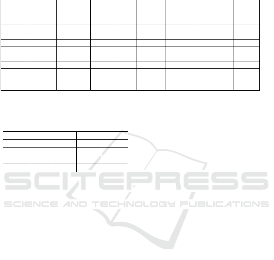
Table 1: Comparison of AQP to state-of-the-art query approximation engines.

Paper

Name

Flat Query

Latency in sec.

(per 1Tb data)

Guaranteed

Error Bound

GPU

Support

Training

Requirement

Preprocessing/

Sampling

Requirement

Queries’ Batch

Concurrent

Processing

Support

Result

Confidence

(28) (29) Hive Hadoop 400 no yes no yes yes NA

(30) (28) Hive Spark 40 no yes no yes yes NA

(31) (11) BlinkDB 2 2-10% no no yes yes 95%

(10) (32) SnappyData 1.5 NA no no yes yes NA

(23) (21) VerdictDB 1 2.6% no no yes yes 95%

(33) (34) DICE 0.5 10% no no yes no NA

(14) DeepGen NA 0.1-1.25% yes yes yes yes No

(15) ML AQP 20 1-5% no yes yes no NA

ur Method AQP 10 <2.5% yes yes yes yes NA

This query was extracted from the results of the

Group By query as seen in Table 2.

Table 2: An example of a ‘Group by’ result set.

city

gender avg(age) max(age)

New York male 51.8 92.5

London male 48.2 89.5

New York female 52.9 94.2

London female 49.1 96.1

3.2 Generating Training Set

To train a deep NN the method generates a large

training set of queries. We used multiple steps which

are described ahead to create a representative training

set of SQL queries. The query template consists of:

(1) the ’SELECT’ clause parameters, (2) the filter

template (i.e., the WHERE clause parameters), and

(3) the name(s) of the table(s). In this phase, the set of

aggregation functions paired with a set of target data

columns is defined. The method then constructs a

’SELECT’ clause consisting of the selected

aggregation functions, which are applied on a set of

the target data columns {a

(col

)}.

All of the aggregation functions can be applied on

numeric data columns, however, the only aggregation

functions that can be applied on discrete columns are

′

count

′

and

′

countDistinct.

′

In our example, assuming

that the domain expert chooses to apply all of the

aggregation functions A on all valid {a

(col

)}, the

result is the following ’SELECT’ clause:

SELECT avg(’Life expectancy’), max(’Life expectancy’)

As mentioned, each {a

(col

)} will have a

designated model that will be trained to learn its

unique distribution. This means that the training set

will be split for each {a

(col

)} and will be learned

separately. In our example, the first training set will

consist of queries with avg(’Life expectancy’) in the

’SELECT’ clause, the second training set will consist

of queries with MEDIAN(’Life expectancy’) and so

on. Next, a filter is defined that includes the list of

numeric data columns col

(n)

and discrete data columns

col

(n)

. Then, for each defined querytemplate, the

method generates a set of queryinstances as follows.

3.3 Formulating Filters

Here, the method generates filters consisting of (1)

numeric data columns col

(n)

, and (2) discrete data

columns col

(n)

in the following manner:

1) For each col

(n)

, our methods calculate the

intervals defined by the minimum value, the first

quartile (25%), the median, the third quartile

(75%), and the maximum value (four intervals).

To select the lower and upper bounds of a

numeric column constraint

range

col

(

(f,c), we

select two intervals randomly. Then, from each

selected interval, we randomly choose a value

sampled from a uniform distribution. This

process results in two numeric values that form

a filter, range_col

(n)

(f,c) such that the smaller

value will define the lower bound and the larger

value will define the upper bound, for example

range

income

(10125,81590).

2) To construct a discrete filter, our method uses an

"IN" constraint argument defined on a discrete

data column col

(n)

, filtered by v

, which is a list

of possible members of col

(n)

. To determine

which member to use in each filter, the method

constructs a ‘Group by’ term on the discrete

columns. Once the query is executed against the

dataset, the method systematically extracts all

possible combinations of members that exist in

the result set and constructs a discrete filter for

each combination. In our example, this is one

IDAT: An Interactive Data Exploration Tool

607

possible combination of the members for city

and gender:

{exist

city

(

′

NewYork

′

),exist

gender

(

′

Male

′

)}.

3) Finally, each combination of discrete filters is

paired with each of the numeric filters to form a

query filter; for example,

{range

income

(10125,81590),exist

city

(‘NewYork

′

),exist

gender

(‘Male

′

)}.

3.4 Generating ‘JOIN’ Clause

In this step, a join clause is added to the query. iDat

supports ’INNER’ and ’OUTER’ joins (left and

right). The join key is configured within the schema

configuration files and is taken to build the ’JOIN’

syntax in the following format:

{join_type

left_table

(left_key),right_table(right_key)}

where join_type can contain the values: (1)

INNER, (2) LEFT, (3) RIGHT and (4) CROSS (for

the last option key is not relevant) e.g.

life_exp ls

RIGHT OUTER JOIN geo_country gc ON ls.city =

gc.c_code

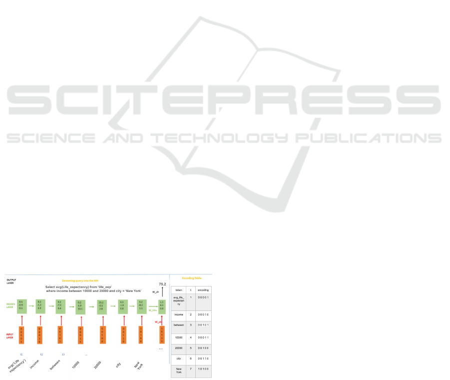
3.5 Embedding Layer Encoder

This phase’s goal is to transform string SQL queries

to numeric matrices. At this stage, a list of ‘flat’ SQL

queries and their real labels (result) is available. Since

RNN can only receive numeric input, we encode the

queries into an embedding space, which produces

numeric matrices (see Figure 1). For that, we use an

encoder model that is constructed on the fly (during

SQL query generation), making use of a multi-hot

encoding technique. The encoding process starts by

mapping all unique query tokens that exist in the

training set Q and assigning each a sequential numeric

value, as illustrated in Figure 1 (for example, the

token avg (’Life expectancy’) is assigned to the value

00001). Each numeric value is then transformed into

a binary numeric representation (base 2). Numeric

query tokens (scalars) are also transformed into their

binary (base 2) representation.

Figure 1: Inducing an embedding layer encoder.

3.6 Training Set Labels

As the goal of the second phase to acquire training set

labels, iDat must run the queries in the database to get

real results. We used Postgres DB to run these

queries. The characteristics of the data sets, their

footprint, and other important statistical metrics are

shown in Table 3.

3.7 NN Training

In the last stage, the algorithm pipeline builds a

sequential NN network (RNN). We chose sequential

NN (i.e. RNN) since this method have been shown to

be efficient in learning complex sequential data,

which was our initial motivation for selecting this

architecture (Lipton et al., 2015).

3.8 Data Changes

To handle new data entering the data base, we build a

hybrid retrain set of SQL queries that will consist of

newly inserted data records and old data records that

have been learned by the model. This is described in

the following method:

1) Time reference - Mark data records with insert

date-time column referred as "insert_dt" and

model training datetime refereed to as

"model_train_dt".

2) Small retrain set - Using the above-mentioned

date-time columns, build a relatively small

retrain set of SQL queries that will span both

newly inserted records and existing records.

3) Query split - split each query to two queries

according to the "model_train_dt":

a) "model_query" - this query will impute a filter

which is less than "model_train_dt". Acquire

a label for these queries by running a query

against the existing model.

b) "data_query" - this query will impute a filter

which is equal or greater than "model_

train_dt". Acquire a label for these queries by

running a query against the data base.

4) Query merge - "model_query" and "data_query"

results according to aggregation function logic:

If "Sum" function is used, sum results of the

queries, if "Average" function is used, calculate

weighted (by the count of records from each

query) average, if "Count" function is used, sum

up the counts, and if "Min/Max" is used, take

one of the values from the 2 queries according to

the function logic.

5) Retrain - Run retrain task on the merged SQL

query set.

DATA 2025 - 14th International Conference on Data Science, Technology and Applications

608

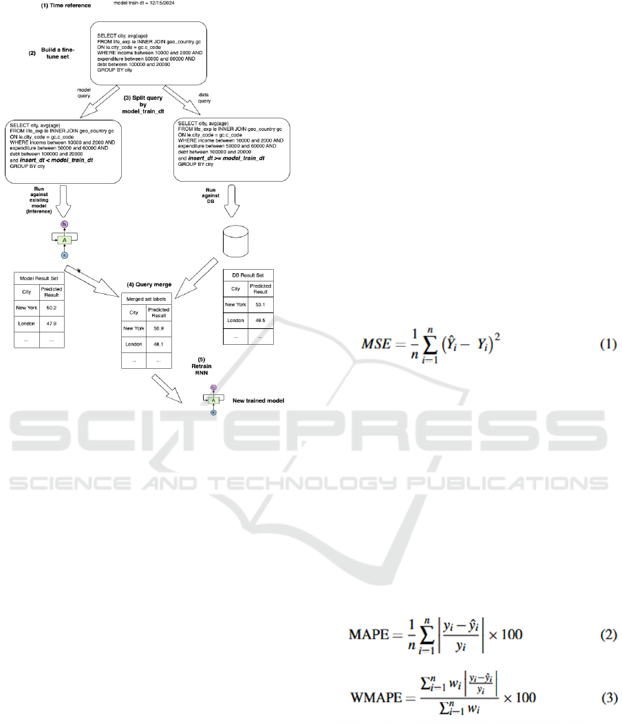
Figure 2: AQP data changes adaptation method.

4 EVALUATION

For evaluation we gathered a group of 20 data

scientists working in leading technology companies

and requested each to provide a set of 10 data

exploration queries for each of the following data sets.

Then, we acquired the queries predictions from iDat

and evaluated the results in terms of accuracy and

latency, as described above.

4.1 Data Sets

The system was evaluated using 12 unique datasets,

both proprietary and open source. The characteristics

of the data sets are presented in Table 3.

4.2 Training Sets Partition

For each dataset, a training set was generated and

split, using the sklearn cross_validation (˙train_

test_split) Python package, into three datasets:

(1) training set - 70% of the queries, (2) validation set

- 15%, and (3) testing set - 15%.

4.3 Handling Overfitting

To avoid overfitting, i.e., a scenario in which the

model memorizes the training set and does not

generalize to the test set, the following steps were

performed: (1) All RNN models (for each dataset)

were validated during optimization (backpro-

pagation) on a randomly selected hold-out set (i.e., the

validation set). (2) After the last training epoch, we

obtained the evaluation metric values for the

inferences made on a second hold-out set (i.e., the test

set), which was randomly selected before the training

took place. (3) Steps 1 and 2 were repeated 30 times,

and the average was used when evaluating our

method’s performance on each metric.

4.4 RNN Cost Function

The RNN network was trained to minimize a

quadratic cost function defined as:

Where Y

is the real query result, Yˆ

is the model’s

approximated query result, and n is the batch size.

4.5 Evaluation Metrics

Since the target variable (query result) is continuous,

the RMSE regression might be a natural candidate for

a cost function, however it can yield an un-normalized

range of values and is greatly influenced by the

problem’s scale. For this reason, we sought a robust

loss metric that would allow us to compare

performance between data sets with significantly

different distributions. To achieve this, we opted to use

a normalized metric: MAPE and weighted MAPE,

defined as follows:

Where i represents a query from the test set, Yi is the

real query result, Yˆi is the model’s approximated

query result, and n is the size of the validation set, and

wi is the weight for the i-th query, which is

proportional to the row count of Yi.

In addition we measured the model performance

based on the time elapsed to perform a SQL query

prediction as described ahead:

IDAT: An Interactive Data Exploration Tool

609

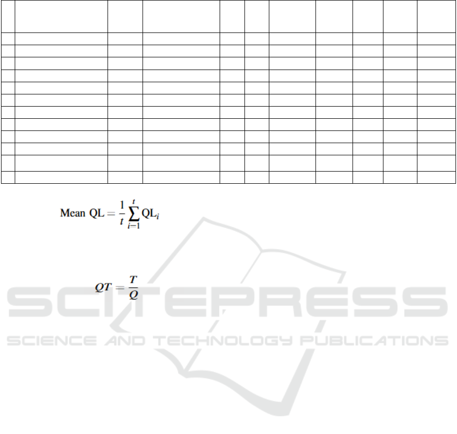
Table 3: Datasets’ characteristics.

Dataset

Proprieta

ry data

source

Target function

attr(n)

attr(c) # rows # queries

Mean

entrop

Input

tensor

variance

Target

column

STD

1 average_revenue Yes avg (revenue) 3 2 1000000000 5205078 6.293 0.154 40400000

2 average_success_rate Yes

avg (build_time)

2 3 2333293 415791 2.264

5.421 19.196

3 count_product_pass Yes count (machine_id) 1 5 4000000000 811928 0.942 0.151 2350516

4 count_product_fail Yes count (machine_id) 1 5 95484 451173 0.942 0.153 8613

5 count_product_false_calls Yes

count (machine_id)

1 5 350232 378111 0.942

0.202 215315

6 count_churn_customers Yes count (customer_id) 4 3 9263836 62092 2.782 0.13267 530

7 sum_duration_call Yes sum (duration) 3 2 9349 100000 3.198 0.167 861

8 average_ibm_price No

avg (close_price)

1 2 1048575 340489 0.343

0.125 471

9 average_realestate_price No avg (price) 3 2 22489348 508086 2.113 0.105 236

10 avg_stock_close_price No avg (close_price) 2 1 63267 8721 5.703 0.157 118

11 average_paid_days Yes

avg(actual_paid_days)

3 2 100000000 508365 0.451

0.099 25667553

12 average_build_duration Yes avg (duration) 1 3 22276094 325935 0.993 0.129 7487

(4)

Where t is the total number of validation queries and

QLi is the Query Latency for the i-th query, measured

in ms.

( 5)

In addition, we calculated the queries’ throughput

(using the GPU to approximate a batch of queries),

which is referred to as QT:

Where T is the total latency of the batch mode

prediction operation, and Q is the number of queries

used in the testing set.

4.6 Benchmark Methods

We compare our method to two state-of-the-art

methods: (1) VerdictDB (Mozafari et al., 2018), a

novel AQP method that accelerates analytical queries,

and (2)

BlinkDB (Agarwal and Mozafari, 2013) - an

approximate query engine for running interactive

SQL queries on large volumes of data. We use the

mean query latency (QL) and WMAPE metrics to

evaluate performance and accuracy respectively.

5 EXPERIMENTAL RESULTS

For each dataset, Table 4 specifies the RNN network

training parameters and the trained models’

performance metrics. These results were gathered

from the execution of SQL queries source from the

group of 20 data scientists taking part in this study.

5.1 Accuracy

As expected, the WMAPE value for the largest

models (datasets number 1,4,8), with RNN layer with

512 neurons and a dense layer with 400 neurons, was

the lowest (most accurate), with a range from of 1-

1.5%, while for the smallest model (dataset number

6), RNN layer with 128 neurons and a dense layer

with 200 neurons, was the highest, with a value of

3.48 (least accurate).

5.2 Query Latency Performance

In dataset number 10, using the GPU, iDat performed

a throughput (QT) of approximately 120K (with a

large batch of 2048) queries per second was

measured, while in dataset number 4, a single query

latency (QL) for our largest (slowest) model lasted

approximately 32 ms.

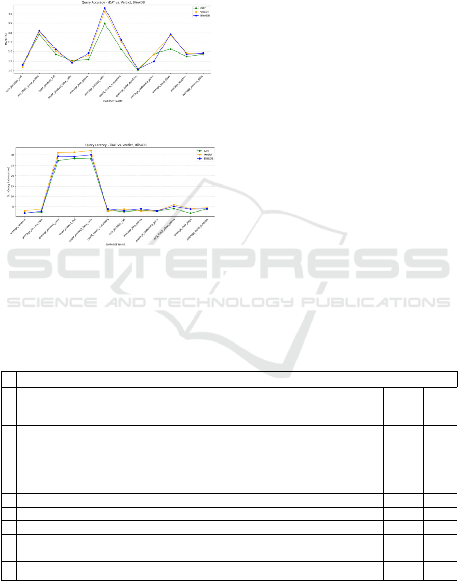
5.3 Benchmark Comparison Results

Figures 4 and 3 depict the accuracy and latency of

iDat and the benchmark methods, VerdictDB

(Mozafari et al., 2018), and BlinkDB (Agarwal and

Mozafari, 2013), on all the datasets. Figure 5 presents

the results of a nonparametric paired Ttest analysis

used to determine if our method is statistically better

than the compared benchmarks in terms of accuracy

(WMAPE) and query latency (mean QL). From this

analysis it is evident that our method was superior for

the majority of the datasets examined (both on the

accuracy and latency metrics), however these

DATA 2025 - 14th International Conference on Data Science, Technology and Applications

610

differences were not statistically significant. In

addition, we evidently show that iDat method can be

used in the field by data scientists to perform data

exploration task on very large data sets.

Figure 3: Comparing the accuracy (WMAPE) performance

of iDat with Verdict and Blink.

Figure 4: Comparing the query latency (mean QL)

performance of iDat with Verdict and Blink.

6 DISCUSSION

Our method in this study predicts the results of the

query within a controlled error (WMPAE), ranging

between 1% to 4%, QL ranges from 2 ms/q to 32

ms/q for a single query. Moreover, for large datasets

(20M - 4B records), our method is two orders of

magnitude faster than the benchmarks used in our

comparison. Based on these encouraging results, we

began to consider the proposed method a novel data

exploration tool for data scientists, capable of

reducing heavy lifting database processing and

reducing incurred storage and scanning costs. Our

method can also predict missing data points or data

points that span into the future e.g. see 10

dataset

(avg_stock_close in Table 3) obtained an WMAPE of

approximately 0.2% for the testing set with future

dates. From the perspective of scale, compared with

other state-of the-art methods, our method can scale

to large datasets (>2M rows) mainly because our

method decouples the data from the query layer once

training finishes. Finally, our method has the

advantage of being lean (2.7Mb on average). This

enables fast inference (query predictions) and

deployment in client production clusters.

However, there are few shortcomings of our method

as follows:

1) Training set generation - generating a set of SQL

queries with a reference to a dataset might not

always represent the user queries’ requirements.

2) Sampling data to generate query filters might

shift the model toward representation of queries

that span on the sampled data on the expense of

data which was not sampled.

3) Initial training time - When our method is trained

for the first time, training may last up to 12

hours.

Table 4: Model performance and accuracy metrics on the datasets.

RNN architecture and hyper-parameters Model performance

# Dataset name

Batch

size

RNN

neurons

Dense

neurons

Input

shape

GPU Type

(q/s)

(ms/q)

WMAPE

RNN

size(Mb)

1 average_revenue

1.E-05 2048 512 400 (7,17) GTX 2060 24398 2.61 1.75 3.47

2 average_success_rate

1.E-02 1024 128 200 (7,17) GTX 2060 42974 2.46 3.48 2.38

3 count_product_pass

1.E-04 2048 512 400 (16,18) GTX 2060 1911 27.37 1.87 3.75

4 count_product_fail

1.E-03 1024 512 400 (16,18) AWS K80 6071 28.41 2.10 3.75

5 count_product_false_calls

1.E-04 1024 512 400 (16,18) AWS K80 1798 28.17 1.52 3.75

6 count_churn_customers

1.E-02 2048 128 200 (17,17) AWS K80 20854 3.45 2.11 2.54

7 sum_duration_all

1.E-02 512 512 400 (7,20) GTX 2060 1982 3.77 1.21 3.61

8 average_ibm_price

1.E-02 128 256 200 (7,62) AWS K80 25681 3.35 1.59 2.91

9 average_realestate_price

1.E-02 1024 128 200 (13,61) GTX 2060 74071 2.90 1.87 2.81

10 avg_stock_close_price

1.E-02 2048 128 200 (6,61) GTX 2060 120288 4.14 3.10 2.95

11 average_paid_days

1.E-05 2048 128 200 (27,7) AWS k80 60074 2.01 2.13 2.62

12 average_build_duration

1.E-04 1024 256 200 (10,32) GTX 2060 11956 3.95 1.02 2.71

IDAT: An Interactive Data Exploration Tool

611

7 CONCLUSION

The primary goal of this research was to implement a

novel approach for EDA scenarios for the practical

use of data scientists and analysts. Existing query

methods require ongoing access to the underlying

data. Once training has taken place, our proposed

method does not require an on-line connection to the

data to explore the data. This opens a variety of

potential use cases for big data analytics.

REFERENCES

Acharya, S., Gibbons, P. B., Poosala, V. and Ramaswamy,

S. “The aqua approximate query answering system,” in

Proceedings of the 1999 ACM SIGMOD international

conference on Management of data, 1999, pp. 574–576.

Agarwal, S., Iyer, A. P., Panda, A., Madden, S., Mozafari,

B. and Stoica, I., “Blink and it’s done: interactive

queries on very large data,” ACM, 2012.

Agarwal, S., Milner, H., Kleiner, A., Talwalkar, A., Jordan,

M., Madden, S., Mozafari, B. and Stoica, I., “Knowing

when you’re wrong: building fast and reliable

approximate query processing systems,” in

Proceedings of the 2014 ACM SIGMOD International

Conf. on Management of data, 2014, pp. 481–492.

Agarwal, S., Mozafari, B., Panda, A., Milner, H., Madden,

S. and Stoica, I., “Blinkdb: queries with bounded errors

and bounded response times on very large data,” in

Proceedings of the 8th ACM European Conf. on

Computer Systems, 2013, pp. 29–42.

Babcock, B., Datar, M. and Motwani, R., “Sampling from

a moving window over streaming data,” in 2002 Annual

ACM-SIAM Symposium on Discrete Algorithms (SODA

2002). Stanford InfoLab, 2001.

Bagchi, A., Chaudhary, A., Eppstein, D. and Goodrich, M.

T., “Deterministic sampling and range counting in

geometric data streams,” ACM Transactions on

Algorithms (TALG), vol. 3, no. 2, pp. 16–es, 2007.

Chandramouli, B., Goldstein, J., Barnett, M., DeLine, R.,

Fisher, D., Platt, J. C., Terwilliger, J. F. and Wernsing,

J. “Trill: A high-performance incremental query

processor for diverse analytics,” Proceedings of the

VLDB Endowment, vol. 8, no. 4, pp. 401–412, 2014.

Chaudhuri, S., Ding, B. and Kandula, S. “Approximate

query processing: No silver bullet,” in Proceedings of

the 2017 ACM International Conference on

Management of Data, 2017, pp. 511–519.

Chuang, K.-t., Chen, H.-l. and Chen, M.-s., “Feature-

preserved sampling over streaming data,” ACM

Transactions on Knowledge Discovery from Data

(TKDD), vol. 2, no. 4, pp. 1–45, 2009.

Cormode, G., Garofalakis, M., Haas, P. J. and Jermaine, C.,

“Synopses for massive data: Samples, histograms,

wavelets, sketches,” Foundations and Trends in

Databases, vol. 4, no. 1–3, pp. 1–294, 2012.

Cuzzocrea A. and Saccà, D., “Exploiting compression and

approximation paradigms for effective and efficient

online analytical processing over sensor network

readings in data grid environments,” Concurrency and

Computation: Practice and Experience, vol. 25, no. 14,

pp. 2016–2035, 2013.

Dokeroglu, T., Ozal, S., Bayir, M. A., Cinar, M. S. and

Cosar, A., “Improving the performance of hadoop hive

by sharing scan and computation tasks,” Journal of

Cloud Computing, vol. 3, no. 1, p. 12, 2014.

Galakatos, A., Crotty, A., Zgraggen, E., Binnig, C. and

Kraska, T. “Revisiting reuse for approximate query

processing,” Proceedings of the VLDB Endowment,

vol. 10, no. 10, pp. 1142–1153, 2017.

Gibbons, P. B., Matias, Y. and Poosala, V., “Fast

incremental maintenance of approximate histograms,”

in VLDB, vol. 97. Citeseer, 1997, pp. 466– 475.

He, W., Park, Y., Hanafi, I., Yatvitskiy, J. and Mozafari, B.,

“Demonstration of verdictdb, the platform-independent

aqp system,” in Proceedings of the 2018 International

Conf. on Management of Data, 2018, pp. 1665–1668.

Jagadish, H. V., Koudas, N., Muthukrishnan, S., Poosala,

V., Sevcik, K. C. and Suel, T., “Optimal histograms

with quality guarantees,” in VLDB, vol. 98, 1998, pp.

24–27.

Jayachandran, P., Tunga, K., Kamat, N. and Nandi, A.,

“Combining user interaction, speculative query

execution and sampling in the dice system,”

Proceedings of the VLDB Endowment, vol. 7, no. 13,

pp. 1697– 1700, 2014.

Kamat, N., Jayachandran, P., Tunga, K. and Nandi, A.,

“Distributed and interactive cube exploration,” in 2014

IEEE 30th International Conference on Data

Engineering. IEEE, 2014, pp. 472–483.

Li K. and Li, G., “Approximate query processing: What is

new and where to go?” Data Science and Engineering,

vol. 3, no. 4, pp. 379–397, 2018.

Li K. and Li, G., “Approximate query processing: What is

new and where to go?” Data Science and Engineering,

vol. 3, no. 4, pp. 379–397, 2018.

Lipton, Z. C., Berkowitz, J. and Elkan, C., “A critical

review of recurrent neural networks for sequence

learning,” arXiv preprint arXiv:1506.00019, 2015.

Mozafari B. and Niu, N., “A handbook for building an

approximate query engine.” IEEE Data Eng. Bull., vol.

38, no. 3, pp. 3–29, 2015.

Mozafari, B., Ramnarayan, J., Menon, S., Mahajan, Y.,

Chakraborty, S., Bhanawat, H. and Bachhav, K.

“Snappydata: A unified cluster for streaming,

transactions and interactice analytics.” in CIDR, 2017.

Nguyen H. S. and Nguyen, S. H., “Fast split selection

method and its application in decision tree construction

from large databases,” International Journal of Hybrid

Intelligent Systems, vol. 2, no. 2, pp. 149–160, 2005.

Park, Y., Mozafari, B., Sorenson, J. and Wang, J.,

“Verdictdb: Universalizing approximate query

processing,” in Proceedings of the 2018 International

Conf. on Management of Data, 2018, pp. 1461–1476.

Ramnarayan, J., Mozafari, B., Wale, S., Menon, S., Kumar,

N., Bhanawat, H., Chakraborty, S., Mahajan, Y.,

DATA 2025 - 14th International Conference on Data Science, Technology and Applications

612

Mishra, R. and K. Bachhav, “Snappydata: A hybrid

transactional analytical store built on spark,” in

Proceedings of the 2016 International Conf. on

Management of Data, 2016, pp. 2153–2156.

Regev, N., Rokach, L. and Shabtai, A. “Approximating

aggregated SQL queries with LSTM networks,” in

2021 International Joint Conf. on Neural Networks

(IJCNN). IEEE, 2021, pp. 1–8.

Savva, F., Anagnostopoulos, C. and Triantafillou, P., “Ml-

aqp: Querydriven approximate query processing based

on machine learning,” arXiv preprint arXiv:

2003.06613, 2020.

Sivarajah, U., Kamal, M. M., Irani, Z. and Weerakkody, V.

“Critical analysis of big data challenges and analytical

methods,” Journal of Business Research, vol. 70, pp.

263–286, 2017.

Slęzak, D., Glick, R., Betlínski, P., and P. Synak, “A new

approximate´ query engine based on intelligent capture

and fast transformations of granulated data summaries,”

Journal of Intelligent Information Systems, vol. 50, no.

2, pp. 385–414, 2018.

Thirumuruganathan, S., Hasan, S., Koudas, N. and Das, G.,

“Approximate query processing using deep generative

models,” arXiv preprint arXiv:1903.10000, 2019.

Thirumuruganathan, Saravanan, et al., “Approximate query

processing for data exploration using deep generative

models,” in 2020 IEEE 36th International Conference

on Data Engineering (ICDE). IEEE, 2020, pp. 1309–

1320.

Todor, B., Ivanov; Max-Georg, “Evaluating hive and spark

sql with bigbench,” Arxiv.org, 2016.

Zaharia, M., Das, T., Li, H., Hunter, T., Shenker, S. and

Stoica, I. “Discretized streams: Fault-tolerant streaming

computation at scale,” in Proceedings of the twenty-

fourth ACM symposium on operating systems

principles, 2013, pp. 423–438.

Zeng, K., Agarwal, S., Dave, A., Armbrust, M. and Stoica,

I. “G-ola: Generalized on-line aggregation for

interactive analysis on big data,” in Proceedings of the

2015 ACM SIGMOD International Conference on

Management of Data, 2015, pp. 913–918.

IDAT: An Interactive Data Exploration Tool

613