Predictors of Freshmen Attrition: A Case Study of Bayesian Methods

and Probabilistic Programming

Eitel J. M. Laur

ıa

School of Computer Science and Mathematics, Marist University, Poughkeepsie, New York, U.S.A.

Keywords:

Bayesian Methods, Probabilistic Programming, Freshmen Attrition, Higher Education Analytics.

Abstract:

The study explores the use of Bayesian hierarchical linear models to make inferences on predictors of fresh-

men student attrition using student data from nine academic years and six schools at Marist University. We

formulate a hierarchical generalized (Bernoulli) linear model, and implement it in a probabilistic program-

ming platform using Markov chain Monte Carlo (MCMC) techniques. Model ﬁtness, parameter convergence,

and the signiﬁcance of regression estimates are assessed. We compared the Bayesian model to a frequentist

generalized linear mixed model (GLMM). We identiﬁed college academic performance, ﬁnancial need, gen-

der, tutoring, and work-study program participation as signiﬁcant factors affecting the log-odds of freshmen

attrition. Additionally, the study revealed ﬂuctuations across time and schools. The variation in attrition rates

highlights the need for targeted retention initiatives, as some schools appear more vulnerable to higher at-

trition. The study provides valuable insights for stakeholders, administrators, and decision-makers, offering

applicable ﬁndings for other institutions and a detailed guideline on analyzing educational data using Bayesian

methods.

1 INTRODUCTION

In higher education, the issue of student dropout rates

has always remained a serious concern, and its effects

extend well beyond the academic domain. Poor re-

tention of students has negative effects on the pres-

tige and the ﬁnancial stability of an educational in-

stitution. At a time when students and their families

often feel that a college education is too expensive

and has uncertain outcomes and return of investment,

schools must, more than ever, track how many and

why students leave their programs. Student attrition

rates are especially high during the freshman year,

which places the focus on addressing the transition

of traditional freshmen students during their ﬁrst year

of college and into their sophomore year. Accord-

ing to the National Center for Educational Statistics

(NCES, 2022), for students who entered a 4-year in-

stitution in Fall 2019, the overall retention rate was

82%, with a wide spread between the more selective

and less selective institutions. At public 4-year in-

stitutions the retention rate was 82% overall, 96% at

the most selective institutions, and 59% at the least

selective institutions. Similarly, at private non-proﬁt

institutions, the retention rate was 81% overall, with

https://orcid.org/0000-0003-3079-3657

92% for the most selective institutions and 64% for

the least selective institutions. In private for-proﬁt

institutions the overall retention rate was 63% At 2-

year degree granting institutions, the overall full-time

freshmen retention rate was 61%, with 61% for pub-

lic institutions, 68% for private nonproﬁt, and 67%

for private for-proﬁt institutions. In comparison, 64%

of students who joined 4-year institution in fall 2014

completed the degree within 6 years, which shows

that a large large percentage of student attrition hap-

pens during or at the end of the freshman year, as

also reported in a number of studies (Deberard et al.,

2004; NSCRC, 2014). But despite all the research

in the academic and learning analytics domain, in-

cluding student performance and retention analysis

(Campbell, 2007; Laur

ıa et al., 2020, for e.g.), and

the widespread availability of technology platforms

and software systems that can learn from data, very

little has been done using the machinery of Bayesian

methods and probabilistic programming. Bayesian

methods have emerged as a more intuitive and robust

alternative to frequentist inference methods, blend-

ing prior beliefs with data to compute probability

distributions of model parameters (Bertolini et al.,

2023). But these methods, techniques and software

tools have received considerable less attention by re-

120

Lauría and E. J. M.

Predictors of Freshmen Attrition: A Case Study of Bayesian Methods and Probabilistic Programming.

DOI: 10.5220/0013555800003967

In Proceedings of the 14th International Conference on Data Science, Technology and Applications (DATA 2025), pages 120-131

ISBN: 978-989-758-758-0; ISSN: 2184-285X

searchers and practitioners in the educational domain,

been mostly relegated to speciﬁc niches -Bayesian

knowledge tracing, used in many intelligent tutoring

systems (Yudelson et al., 2013; Dai et al., 2021), nat-

ural language processing and text mining (Chen et al.,

2022), and to a lesser extent, Bayesian networks (De-

len, 2010). A simple experiment reinforces these as-

sertions: a search on Google Scholar with keywords

student retention (or attrition), predictors, and ma-

chine learning / statistical analysis / data analysis

yields several thousand results. When we replace the

latter with a combination of keywords Bayesian and

MCMC / Markov chain Monte Carlo / variational in-

ference / NUTS (all common terms in a Bayesian in-

ference setting), the number of search results drops

way below one hundred.

This paper explores the use of Bayesian hierar-

chical linear regression models using data from mul-

tiple academic years to derive insights on freshmen

student retention. Hence, the paper makes the fol-

lowing contributions: 1) It frames freshmen retention

analysis through the lens of Bayesian inference. 2)

It describes the use of Bayesian hierarchical linear

models, demonstrating the use of hierarchical mod-

els to account for data organized in multiple layers or

levels; 3) It highlights the computational power and

simplicity of probabilistic programming tools, pro-

viding reproducible data-driven workﬂow practices in

this context. The paper is organized in the following

manner: we start with a section on Bayesian meth-

ods and probabilistic programming, introducing key

concepts and their application to modeling freshmen

attrition. Next, we describe the study, including re-

search questions, data, methods, technology platform,

and results. The paper ends with a summary of our

conclusions.

2 BAYESIAN METHODS AND

PROBABILISTIC

PROGRAMMING

2.1 Overview

Bayesian methods provide a framework to make in-

ferences from data using probability to quantify un-

certainty. Bayesian models are grounded in Bayes’

theorem, which describes the relationship between

the prior or initial beliefs on the probability distribu-

tions of the model parameters, the likelihood func-

tion, and the posterior distribution, the probability of

observing the data given the model parameters, also

known as the likelihood function, and the posterior

distribution of the model parameters, representing the

conditional distribution of the parameters represent-

ing the updated beliefs after observing the data. To

formulate Bayes theorem, let’s consider observable

data X, and a vector of unobservable parameters θ.

Bayes’ theorem is therefore expressed as:

P(θ|X) =

P(X|θ)P(θ)

P(X)

(1)

where P(θ) in Equation 1 is the prior distribution of

vector parameter θ; P(X | θ) is the likelihood of the

data X given θ; P(θ | X) is the posterior distribution

of θ after observing X ; and P(X) =

P(X | θ) p(θ)dθ

is the marginal likelihood of X, which serves as a nor-

malization constant.

Why is the Bayesian framework important? Be-

cause it provides a common-sense, straightforward

interpretation of statistical conclusions. A Bayesian

high-density interval (HDI) for an unknown quantity

of interest provides a range of values where the quan-

tity of interest is most likely to be, given the observed

data and the priors, in contrast to a frequentist conﬁ-

dence interval (CI), which may strictly be interpreted

only in relation to a sequence of repeated experiments

(Gelman et al., 2013). For example, a 95% HDI is

the region of values that contains 95% of the poste-

rior probability mass, whereas the 95% CI means that

approximately 95% of the intervals calculated from

the repeated experiments would contain the quantity

of interest. In frequentist statistics, a p-value sum-

marizes the probability over many trials of observing

the effect on the outcome, whereas Bayesian meth-

ods estimate the posterior probability of the effect

on the outcome after observing the data; the differ-

ence which seems subtle, has led to misinterpretations

that have spread throughout the scientiﬁc literature,

with students, practitioners and researchers mistaking

p-values as posterior probabilities (Greenland et al.,

2016). The p-value is also sensitive to the amount

of observations: a large sample size can give way to

small p-values that can in turn lead to erroneous asser-

tions about signiﬁcant effects. Bayesian methods are

less affected by the size of the sample, as they pro-

vide a full probability distribution of the effect of the

model parameters on the outcome after observing the

data.

2.2 Approximate Bayesian

Computation and Probabilistic

Programming

Bayes rule, as depicted in Equation 1, hides the com-

plexity of computing the marginal likelihood of the

Predictors of Freshmen Attrition: A Case Study of Bayesian Methods and Probabilistic Programming

121

data P(X) =

P(X | θ) p(θ)dθ, which can be cir-

cumvented through the use of conjugate priors -one

where the product of the prior times the likelihood

yields a statistical distribution of the same form (in

the same family) as the prior distribution. The use

of conjugate priors can be advantageous but also re-

strictive, and not a well-grounded hypothesis in many

real-world situations. But when conjugate priors are

not valid, the marginal likelihood P(X) is an integral

that can be difﬁcult or even impossible to compute,

especially over multiple dimensions. Bayesian in-

ference has to resort then to approximate numerical

techniques such as the Markov Chain Monte Carlo

(MCMC) family of algorithms, or variational infer-

ence. MCMC methods such as Metropolis-Hastings

(Hastings, 1970) and Gibbs sampling (Geman and

Geman, 1984), originally derived from statistical me-

chanics, produce samples approximating the sought

posterior distribution using a proposal distribution to

accept or reject those samples -in the case of Gibbs

sampling, the proposal distribution is the conditional

distribution of one parameter given the others, and

there is no rejection step. Hamiltonian Monte Carlo

or HMC (Duane et al., 1987), another popular vari-

ation of Metropolis-Hastings, simulates the Hamil-

tonian trajectory of a particle in a potential energy

ﬁeld, formulating a proposal distribution that renders

more efﬁcient sampling by avoiding random walk be-

havior and reducing the correlation between succes-

sive samples. The NUTS (No-U-Turn Sampler) al-

gorithm (Homan and Gelman, 2014), an extension of

HMC, uses a recursive algorithm that dynamically de-

termines the length of the simulated Hamiltonian tra-

jectory, avoiding backtracks and therefore leading to

better sampling. MCMC sampling methods are the

most common algorithms for Bayesian computation,

but other approaches have been developed as well.

Variational inference (Blei et al., 2017) is an alter-

native and generally more scalable method that ap-

proximates the posterior distribution of the parame-

ters of interest using a surrogate distribution instead

of resorting to sampling, and estimates the parameters

of the surrogate distribution using optimization algo-

rithms (e.g. variations of gradient descent) such that

the resulting distribution resembles as much as possi-

ble the posterior distribution. Variational inference is

usually faster than MCMC, but it can be less accurate

and it can converge to local minima, which further

restricts accuracy. Where do probabilistic program-

ming platforms come into play? They allow for ﬂexi-

ble speciﬁcation of probabilistic models, and provide

the tools to perform Bayesian inference, hiding the

intricate details of approximate Bayesian inference

computation (MCMC and variational inference) so

that researchers and practitioners can focus on model

design, development, and testing, leaving the proba-

bilistic programming platform to handle the compu-

tational details for them. A number of probabilistic

programming platforms have been developed over the

years, among them BUGS (Gilks et al., 1994), JAGS

(Plummer, 2003), Stan (Carpenter et al., 2017) and

PyMC (Abril-Pla et al., 2023), Stan and PyMC are

popular platforms in active development.

2.3 Using Bayesian Methods to Model

Freshmen Attrition

In a Bayesian context, a typical approach to model

student attrition is to use a binary logistic regression,

a generalized linear model where the response vari-

able y, representing whether the student has dropped

out, follows a Bernoulli distribution with parameter

θ, which in turn is a nonlinear (logistic) function

of a linear combination of m scaled predictors (i.e.

∑

j=1

· x

), representing student demographics,

high school and college student activity, characteris-

tics and academic performance. Numeric data is typ-

ically scaled to improve numerical stability and aid

the convergence and speed of computation. To obtain

stable logistic regression coefﬁcients and circunvent

nonidentiﬁability issues due to separation (when a lin-

ear combination of the logistic regression predictors

perfectly predicts the outcome), sparsity, collinearity,

or the inclusion of numerous binary predictors, the lit-

erature prescribes mild regularization through the use

of noninformative or weakly informative priors on the

regression coefﬁcients, by constraining parameter es-

timates so that they are not too extreme or unrealistic

(Gelman et al., 2008; Westfall, 2017). This formu-

lation is known as a ”ﬂat” or ”pooled” model, in the

sense that it does not take into account the structure

associated with potential grouping and nesting of the

data. Educational data is inherently complex, multi-

layered, and nested: students join majors and minors,

which are part of academic units -departments and

schools. Each level within this layered structure has

its own characteristics which can have an effect on

student academic performance and student attrition.

Also, student attrition data has strong temporal com-

ponents, which give way to repeated measurements

of freshmen attrition over multiple academic years,

affected by internal and external factors (e.g., attri-

tion rates affected by COVID-19). Of course, the

immediate solution that comes to mind when deal-

ing with variability among groups is to ﬁt a sepa-

rate regression model for each of the groups. This

”unpooled” approach addresses the issue of consid-

ering the particular characteristics of each group, but

DATA 2025 - 14th International Conference on Data Science, Technology and Applications

122

since a model is ﬁtted independently for each group,

it is difﬁcult to extract ﬁndings that are common to

all groups. Moreover, unpooled models may be con-

strained by the availability of data: there may not

be enough data in particular groups to ﬁt the regres-

sion model. The multi-layered structure of educa-

tional data introduces this additional wrinkle in the

analysis: data can be sparse at each level. Special-

ized majors and minors might have low enrollment

ﬁgures, and new programs might carry limited histor-

ical data. If the analysis examines data using student

demographic characteristics, certain groups and mi-

norities might be highly underrepresented, giving way

to parameter estimates with high variance, or lead to

unstable, very large or potentially inﬁnite regression

coefﬁcients, a phenomenon described as complete,

or quasi-complete separation. Also, models trained

with small amounts of data are prone to overﬁtting

and may not generalize well when applied to new or

unseen data. This is especially critical when apply-

ing frequentist methods on multi-level data (e.g., fre-

quentist logistic regression), as Bayesian models in-

troduce priors that can help mitigate high variance

and bias of regression coefﬁcients as well as separa-

tion issues. Hierarchical models strike a balance be-

tween effects that are group-speciﬁc and those that

apply more broadly across group populations (Gel-

man and Hill, 2006). Although frequentist hierarchi-

cal models (e.g., mixed-effect models or GLMMs) ad-

dress variability among groups, there are key advan-

tages in applying Bayesian hierarchical models com-

pared to frequentist approaches. Bayesian hierarchi-

cal models apply partial pooling through hierarchical

priors, naturally regularizing group-level estimates to-

wards the overall distribution, and therefore prevent-

ing large coefﬁcient estimates in groups with small

counts. Frequentist hierarchical models can incorpo-

rate regularization, but it is not inherently built in. In

small groups, frequentist models may struggle to ac-

curately estimate the variance of random effects (e.g.

how much of the variability in attrition is due to differ-

ences between schools). On the downside, Bayesian

hierarchical models are computationally more expen-

sive, especially for large datasets, than their frequen-

tist counterparts, which rely on optimization methods

such as maximum likelihood estimation (MLE).

3 STUDY DESIGN

In this study, we investigate the use of Bayesian gen-

eralized linear models to ascertain potential predictors

of freshmen attrition drawn from student data. We

built hierarchical binary logistic regression models

using a probabilistic programming platform to com-

pute the posterior probability distributions of the lo-

gistic regression coefﬁcients and derived metrics. The

quality of the ﬁtted models and the signiﬁcance of the

regression coefﬁcients are measured using the metrics

described in section 2.3.2. We also analyze random

effects due to variability in the different academic

years under study and across different schools within

the academic institution. In doing so, the study ad-

dresses the following research questions:

RQ1: How do student demographics, high school and

university academic performance, and student activi-

ties affect the odds of freshmen attrition?

RQ2: Is there considerable ﬂuctuation in freshmen at-

trition across different academic years and among dif-

ferent schools?

RQ3: How does the Bayesian hierarchical model

compare to its frequentist counterpart?

3.1 Datasets

We considered Freshmen data from nine academic

years (2012-2018, and 2021-2022) extracted from the

institution’s data warehouse. We decided to skip

(2019-2020) data as it corresponds to the COVID-

19 pandemic period, which could introduce variabil-

ity in the results (we are aware that 2021 and 2022

data could be also different from the pre-pandemic

years, but we performed preliminary testing and did

not ﬁnd signiﬁcant variation). See Table 1 for details.

School codes correspond to the following schools:

CC - Computer Science & Mathematics; CO - Com-

munications & the Arts; LA - Liberal Arts; SB - So-

cial & Behavioral Sciences; SI - Science; SM - Man-

agement.

Data was imputed using K-nearest neighbors

(KNN). Each record corresponds to each accepted

and registered freshman student in the Fall of the cor-

responding academic year, enriched with school data

and demographics using the record format depicted

in Table 1. The dataset included 10921 records, with

1154 instances of attrition. Dropouts are considered

over the full academic year (institutional research data

was used to determine if a student who came in in

the Fall of a given academic year, did not return in

the Fall of the following academic year). The over-

all attrition ratio in the dataset was 10.57%. Dataset

was checked to identify outliers and inﬂuential obser-

vations. Numeric variables were scaled as z-scores.

Correlations among predictors were checked: Effec-

tiveGPA correlates with HSGPA (0.49), isDeanList

(0.59), and NumAPCourses (0.26), indicating a rela-

tionship between past and current academic perfor-

mance. EFC (Expected Family Contribution) is neg-

Predictors of Freshmen Attrition: A Case Study of Bayesian Methods and Probabilistic Programming

123

atively correlated with UnmetNeed (-0.33) and Pel-

lAmount (-0.21), reﬂecting expected patterns in ﬁ-

nancial aid allocation. PellAmount is correlated with

UnmetNeed (0.40), hasLoans (0.19), and isCampus-

WorkStudy (0.23). We also checked the Variance In-

ﬂation Factor (VIF). Predictors had a VIF < 5, mean-

ing multicollinearity is not a major concern. Effec-

tiveGPA had a VIF between 2.5 - 3.0, which warrants

some consideration.

Table 1: Data Description.

Identiﬁer Description

Academic Performance

EffectiveGPA (academic year) Numeric

isDeansList (made it to Dean’s list) Binary (1/0)

TutoringClassCount (classes tutored in) Numeric

HSGPA (high school GPA) Numeric

NumAPCourses (taken during high school) Numeric

Demographics

UScitizen Binary (1/0)

Gender Binary (F, M)

StudentofColor Binary (1/0)

isFirstGeneration (college student) Binary (1/0)

DistanceFromHome (miles) Numeric

Institutional and Enrollment Factors

isCampusWorkStudy Binary (1/0)

isDivisionI (athlete) Binary (1/0)

WaitListed (before admitted) Binary (1/0)

Financial Aid and Need

EFC (Expected Family Contribution, in $) Numeric

UnmetNeed (after ﬁnancial aid, in $) Numeric

HasLoans Binary (1/0)

PellAmount (federal grant, in $) Numeric

AcademicYear Discrete

School ((CC, CO, LA, SB, SI, SM) Discrete

didNotReturnNextFall (response variable) Binary (1/0)

3.2 Statistical Modeling

We built a hierarchical binary logistic regression

model using the predictors depicted in Table 1. We

consider random effects in the model associated with

potential variability in the log-odds of freshmen at-

trition across multiple academic years and different

schools. The model, depicted in Equation 2, includes

varying intercepts for both academic year and school;

AcademicYear

is a group-level effect that captures the

effect on the likelihood of the outcome tied to being

in a particular year. Similarly, b

School

captures the ef-

fect of attending a particular school on the log-odds

of dropping out during or at the end of the freshman

year. Regression coefﬁcient priors are denoted by P

We reﬁned the prior distributions of the model, using

the following criteria:

• The choice of the Intercept’s prior as Normal(-

2.2, 1.0) is based on the approximate 10% at-

trition rate. The intercept represents the log-

odds when all predictors are at the mean value,

as they are scaled as z-scores. Therefore if

P(y = 1) =

Intercept

1+e

Intercept

, when P(y = 1) = 0.10 =⇒

log(0.10/0.90) = −2.2.

• We used StudentT(ν=3, ν=0, σ=2.5) on correlated

predictors or predictors width moderate outliers.

ν=3 allows for some large deviations and σ=2.5

keeps the prior weakly informative.

• We used normal weakly informative priors -

Normal(0,2.5) for all other predictors.

• For group effects (School and AcademicYear),

we used HalfNormal(2.5). A σ = 2.5 allows

for moderate variation while keeping the group-

speciﬁc intercepts within a rather similar scale as

the ﬁxed-effects intercept.

The prior distributions with their calculated val-

ues using the criteria described above are depicted in

Table 2.

AcademicYear

∼ HalfNormal(σ

AcademicYear

)

School

∼ HalfNormal(σ

School

)

AcademicYear

∼ Normal(0, σ

AcademicYear

)

School

∼ Normal(0, σ

School

)

∼ Normal(µ

= −2.2, σ

= 1.0)

∼ P

for j = 1,2, .. .,m

logit = b

AcademicYear

+ b

School

+ b

∑

j=1

θ =

1 + exp(−logit)

y ∼ Bernoulli(p = θ)

(2)

3.3 Probabilistic Programming

Platform

We used Bambi (Capretto et al., 2022) -Bayesian

Model Building Interface, a Python package for gen-

eralized linear models built on top of PyMC (Abril-

Pla et al., 2023) and the ArviZ package for ex-

ploratory analysis (Kumar et al., 2019) to develop and

run the Bayesian logistic regression models and pro-

duce visualizations. The Bayesian models developed

in Bambi used the No U-Turn (NUTS) algorithm to

obtain the posterior distribution samples of the regres-

sion parameters. We chose the NumPyro (Phan et al.,

2019) implementation of the NUTS sampler. Sam-

ples of the posterior distributions for the logistic re-

gression parameters were computed using 4 chains of

5000 samples each, with a warm-up period of 1000

samples for each of the chains (the number of samples

initially discarded until the chain converges to the sta-

tionary posterior distribution). The chains were tested

and no divergences were found in any of the chains of

DATA 2025 - 14th International Conference on Data Science, Technology and Applications

124

Table 2: Prior Distributions for Fixed and Group Effects.

Component Prior Distribution

Fixed Effects

Intercept Normal(µ:-2.2, σ:1.0)

EffectiveGPA StudentT(ν:3.0, µ:0.0, σ:2.5)

isDeansList StudentT(ν:3.0, µ:0.0, σ:2.5)

TutoringClassCount Normal(µ:0.0, σ:2.5)

HSGPA StudentT(ν:3.0, µ:0.0, σ:2.5)

NumAPCourses Normal(µ:0.0, σ:2.5)

USCitizen Normal(µ:0.0, σ:2.5)

Gender Normal(µ:0.0, σ:2.5)

StudentOfColor Normal(µ:0.0, σ2.5)

isFirstGeneration Normal(µ:0.0, σ:2.5)

DistanceFromHome StudentT(ν:3.0, µ:0.0, σ:2.5)

isDivisionI Normal(µ:0.0, σ:2.5)

isCampusWorkStudy Normal(µ:0.0, σ:2.5)

WaitListed Normal(µ:0.0, 9.3792)

EFC StudentT(ν:3.0, µ:0.0, σ:2.5)

UnmetNeed StudentT(ν:3.0, µ:0.0, σ:2.5)

HasLoans StudentT(ν:3.0, µ:0.0, σ:2.5)

PellAmount StudentT(ν:3.0, µ:0.0, σ:2.5)

Group-Level (Random) Effect

AcademicYear (Random Intercept) Normal(µ=0.0, σ

AcademicYear

)

AcademicYear

HalfNormal(σ=2.5)

School (Random Intercept) Normal(µ=0.0, σ

School

)

School

HalfNormal(σ=2.5)

the models created. Convergence of the models was

assessed using

R < 1.01 as the threshold for accept-

able convergence (see the section below for details).

3.4 Model Quality and Performance

Metrics

Several metrics are considered to measure the quality

of the model:

•

R =

n−1

, also known as the Gelman-

Rubin diagnostic, is a measure of the convergence

of the MCMC algorithm.

R computes and com-

pares the variance within chains with the variance

between chains. σ

is the between-variance (the

average of the variances of each of the chains) and

is the within-variance, measuring the variabil-

ity between the means of the chains. A value of

close to 1 is an indication of convergence.

• The high-density interval (HDI) summarizes the

range of most credible values of a parameter

within a certain probability mass. When 95%HDI

includes zero, the regression coefﬁcient is not sta-

tistically signiﬁcant. The literature has also sug-

gested the use 89%HDI, see (Kruschke, 2014) for

example. But we prefer to use the 95% interval

in the study, as it is more conservative and has an

intuitive relationship with the standard deviation

(Easystats, 2024).

• The percentage of 95% HDI within ROPE is a

measure of the practical signiﬁcance of the re-

gression coefﬁcients. ROPE (region of practical

equivalence) corresponds to a null hypothesis for

the model parameters and provides a range of val-

ues for the parameters in question that are consid-

ered good enough for practical matters. The so-

called HDI+ROPE decision rule (Kruschke, 2014)

determines the practical signiﬁcance of the regres-

sion coefﬁcients based on the overlap percentage

between the HDI (95%HDI in this case) and the

ROPE range. A percentage value of overlap closer

to 0 implies that the parameter (regression coefﬁ-

cient in this case) is signiﬁcant. The ROPE range

is context-dependent.

• WAIC (Watanabe, 2010), which stands for widely

applicable information criteria, is used both for

model comparison and to measure the model’s

predictive performance (how well the model per-

forms when making predictions on new data).

WAIC uses the log-likelihood evaluated at the

posterior distribution of the parameter values pe-

nalized by the variance in the log-predictive den-

sity across those posterior samples. It is formu-

lated as WAIC = −2 · (LPPD − penalty), where

LPPD =

∑

i=1

(log(

∑

s=1

P(y

| θ

)) is the log

pointwise predictive density and Var(logP(y

))) is the penalty term that accounts for model

complexity. Note that n is the number of observa-

tions and S is the number of samples of the pos-

terior distribution. WAIC’s range is not bounded;

higher values of WAIC are an indication of better

model predictive performance.

• Pareto-smoothed importance sampling leave-one-

out cross-validation, a mouthful of a name, and

better referred to by the short acronym LOO, is a

newer approach introduced by Vehtari et al. (Ve-

htari et al., 2017) to measure out-of-sample pre-

diction accuracy from a ﬁtted model. It uses a

leave-one-out approach, ﬁtting the model n times,

each time with n − 1 observations. but instead

of re-ﬁtting the model n times, the algorithm

uses importance sampling to estimate the leave-

one-out predictive density. Similar to the case

of WAIC, its formulation is derived from ap-

proximating the posterior predictive distribution:

LOO =

∑

i=1

log



∑

s=1

P(y

|θ

−i

)

ˆw



. The −i in-

dex in θ

−i

is used to denote all samples except

; ˆw

are the Pareto-smoothed importance sam-

pling weights. As in the case of WAIC, LOO is

not bounded; higher values of LOO are indica-

tive of better predictive performance. LOO has

been described as being more robust than WAIC

Predictors of Freshmen Attrition: A Case Study of Bayesian Methods and Probabilistic Programming

125

in the presence of weak priors or inﬂuential obser-

vations.

4 STATISTICAL ANALYSIS AND

RESULTS

We ran the hierarchical logistic regression model -

equation (1)- with the prior distributions depicted in

Table 2. Figure 1 displays, for several predictors, the

trace plots with the sampling paths for each of the

chains, along with the kernel density plots of the pos-

terior distributions elicited from each chain (due to

space restrictions we limited the number of predictors

displayed in the ﬁgure to two). The trace plots show

that the chains have ”mixed” well, with each of the

chains converging to the same posterior distribution

of the regression coefﬁcients of each predictor.

To answer Research Question 1 -measuring the in-

ﬂuence of the predictors on freshmen attrition- we

analyzed the results of the ﬁxed effects of the logis-

tic regression. Table 3 reports the regression coef-

ﬁcients derived from their posterior distributions to-

gether with statistical measures for each of the predic-

tors to assess the quality and convergence of the pos-

terior probability distributions of the regression co-

efﬁcients of the predictors calculated by the MCMC

(NUTS) computation and evaluate the ﬁxed effects of

the predictors on the log-odds of freshmen attrition.

• Mean and SD: The mean and standard deviation

of the posterior distribution of the regression of

each predictor, the coefﬁcient measuring the av-

erage estimated effect (log-odds) of each predic-

tor on the outcome (freshmen attrition), and the

spread of the posterior distribution.

• HDI (2.5% and HDI 97.5%): The credible range

of the regression coefﬁcients, given by the lower

and upper boundaries of the 95% Highest Density

Interval (HDI).

• MCSE Mean: The Monte Carlo Standard Error of

the Mean, which provides a measure of the vari-

ability of the mean estimate due to the ﬁnite sam-

ple size.

• MCSE SD: The Monte Carlo Standard Error of

the Standard Deviation, a measure of the variabil-

ity of the standard deviation due to limited sam-

pling.

• ESS Bulk and ESS Tail: The Effective Sample

Size (ESS) for the bulk and tail of the distribution,

which measures the quality of the sampling of the

bulk and tail regions of the posterior distribution

of each regression parameter. The bulk is where

most of the probability mass lies. The tail regions

hold less probable values.

•

R: The convergence diagnostic. All reported

values were equal to 1.0, which suggests that the

MCMC chains converged and therefore the pos-

terior distributions and the estimates derived from

the sampling process can be considered reliable.

• The percentage of 95%HDI within ROPE was

computed for each of the regression parameters in

the logistic regression models to ascertain the pre-

dictors that signiﬁcantly impacted the log-odds of

freshmen attrition. ROPE was ﬁxed at [-0.2,0.2],

following the recommendations by Kruschke (Kr-

uschke, 2018) for binary logistic regression. The

chosen ROPE range of [-0.2,0.2] is especially ap-

propriate considering that we have a combina-

tion of binary predictors and numeric predictors

scaled as z-scores. The ROPE can be seen then

as a region of values of the regression coefﬁcient

around zero that are considered practically equiv-

alent to having a negligible effect on the log-odds

of the outcome. Hence, by setting the ROPE to [-

0.2, 0.2], we establish the criterion of a negligible

change in the log-odds.

We summarize the key ﬁndings from the poste-

rior distributions of the ﬁxed effects, focusing on pre-

dictors that were found to be statistically signiﬁcant

(95% HDI does not include 0) and practically signif-

icant using the percentage of 95% HDI within ROPE

as a practical signiﬁcance criterion.

Effective GPA at the End of the Academic Year,

with Mean=-0.771 and 95% HDI=[-0.842, -0.698],

is negatively associated with freshmen attrition: a

higher GPA reduces the log-odds of attrition, making

it a statistically and practically signiﬁcant predictor.

High School GPA (HSGPA), with Mean=0.129

and 95% HDI=[0.044, 0.214], suggests that higher

high school GPA values could be associated with

higher attrition odds. However, a substantial per-

centage of the 95% HDI falls within ROPE, making

its practical signiﬁcance questionable. This result is

counterintuitive and warrants further investigation.

Made Dean’s List (isDeansList[1.0]), with

Mean=0.571 and 95% HDI=[0.383, 0.756], is statisti-

cally signiﬁcant and practically signiﬁcant, though its

practical impact remains unclear. Students who make

the Dean’s List appear to have a higher probability

of attrition, a ﬁnding that requires deeper exploration

(e.g. whether this institution was the students’ second

choice, who are seeking their ﬁrst choice to continue

their studies)

US Citizenship (USCitizen[1.0]), with Mean=-

0.271 and 95% HDI=[-0.678, 0.127], suggests that

DATA 2025 - 14th International Conference on Data Science, Technology and Applications

126

Figure 1: KDE plots of the posterior distributions and trace plots for each chain.

U.S. citizens may be less likely to drop out, but this

effect is not statistically signiﬁcant.

UnmetNeed, with Mean=0.370 and 95%

HDI=[0.285, 0.456], is both statistically and practi-

cally signiﬁcant. The positive coefﬁcient indicates a

strong association with freshmen attrition: students

with higher unmet ﬁnancial need face signiﬁcantly

increased odds of leaving the institution.

Gender (Male), with Mean=-0.234 and 95%

HDI=[-0.382, -0.087], suggests that male students are

less likely to leave the institution during or at the end

of their freshman year compared to female students.

Has Loans (HasLoans[1.0]), with Mean=-0.210

and 95% HDI=[-0.357, -0.056], suggests that students

with loans are slightly less likely to drop out.

Campus Work Study (isCampusWorkStudy[1.0]),

with Mean=-0.612 and 95% HDI=[-0.833, -0.389],

suggests that freshmen participating in the campus

work-study program are signiﬁcantly less likely to

leave the institution. This result is both statistically

and practically signiﬁcant.

Division I (isDivisionI[1.0]), with Mean=-0.014

and 95% HDI=[-0.204, 0.179], suggests that Division

I athletes do not exhibit a signiﬁcant difference in at-

trition probability, as the 95% HDI includes 0, making

this effect not statistically signiﬁcant.

Pell Amount, with Mean=-0.181 and 95% HDI=[-

0.262, -0.103], suggests that receiving a Pell Grant is

associated with lower attrition, but the effect is rela-

tively small and may not be practically signiﬁcant.

Student of Color (StudentOfColor[1.0]), with

Mean=0.165 and 95% HDI=[-0.037, 0.360], suggests

that being a student of color is associated with slightly

higher attrition odds, but the effect is not statistically

signiﬁcant.

Tutoring Class Count, with Mean=-1.802 and

95% HDI=[-2.732, -0.990], is both statistically and

practically signiﬁcant, indicating that students who

attend tutoring sessions for their courses are much

less likely to drop out. This suggests a strong pro-

tective effect against attrition.

We performed posterior predictive checks using

ArviZ (Kumar et al., 2019) to measure out-of-sample

predictive accuracy by computing the widely appli-

cable information criteria (WAIC) measure, and the

Pareto-smoothed importance sampling leave-one-out

(LOO) measures. In the case of WAIC, the expected

log pointwise predictive density (elpd waic) is equal

to -3239.53, with SE=66.66. The value is negative

as it is a log-likelihood. Higher values (less nega-

tive) indicate better predictive performance. The ef-

fective number of parameters (p waic), with a value

of 28.35, measures model complexity. As the value is

rather small, the measure signals that the model is not

too complex. In the case of LOO, elpd loo and p loo

and very close to the WAIC: elpd loo=-3239.44), with

SE=66.66, and p loo=28.04. This makes the mea-

sures of posterior predictive accuracy and model com-

plexity consistent. ArviZ also reports LOO κ diag-

nostics ( see Table 4). The κ parameter refers to the

shape parameter κ of the Pareto distribution. If all the

records, like in this case, fall within the acceptable

(”good”) range, it means that the importance sam-

pling used when computing LOO is stable, and not

inﬂuenced by particular observations, and therefore

the metric is reliable.

To address Research Question 2, concerning

the ﬂuctuation in ﬁrst-year student retention across

schools and over time, We began by looking at the

distribution of attrition by school and academic year,

as depicted in Figure 2. Both charts display some dif-

ferences in the attrition rate. For attrition distribution

by academic year, year 2021 carries the larger per-

centage of attrition, probably since 2021 marked the

end of the COVID pandemic. In the case of distribu-

tion of attrition by School, the attrition percentage is

smaller in the School of Computer Science & Mathe-

matics (CC), with larger values in Liberal Arts (LA).

We then proceeded to examine the variability in

attrition rates by studying random effects for aca-

Predictors of Freshmen Attrition: A Case Study of Bayesian Methods and Probabilistic Programming

127

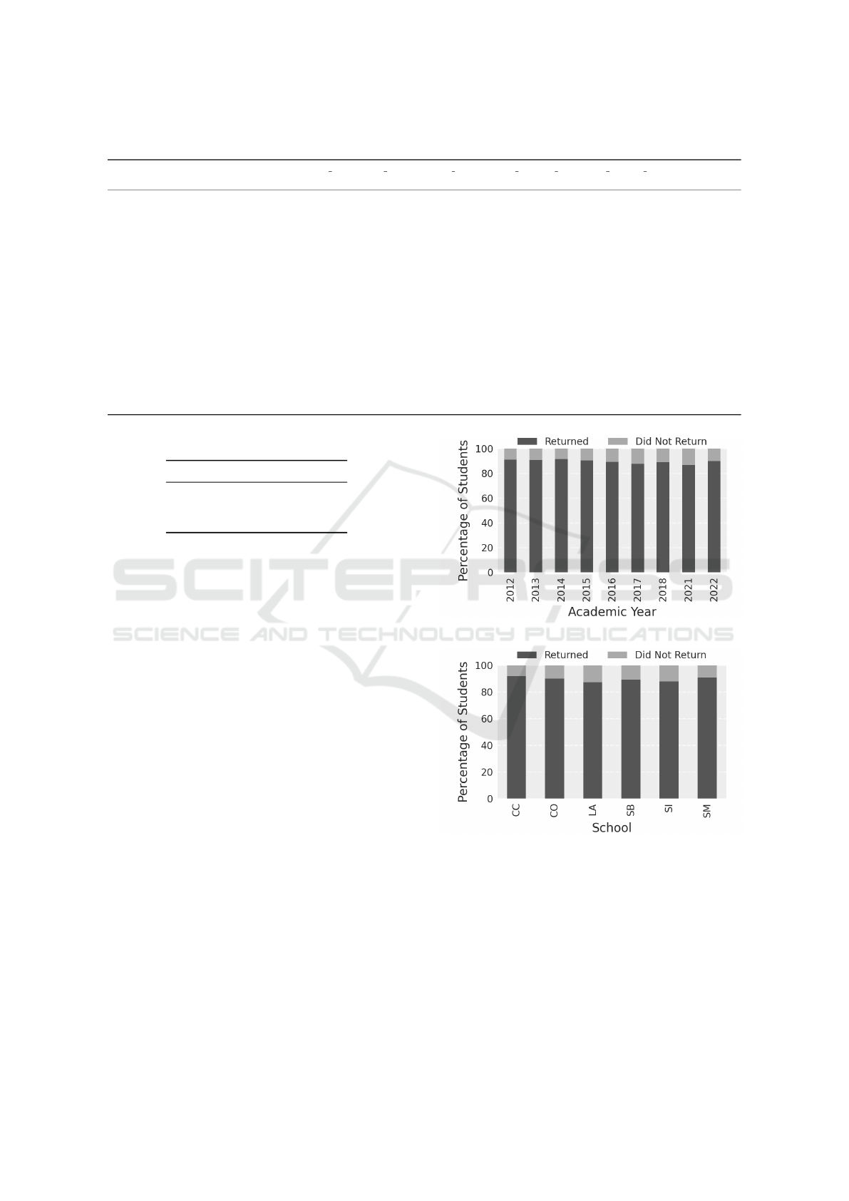
Table 3: Summary of Posterior Distributions.

Component mean sd hdi 2.5% hdi 97.5% mcse mean mcse sd ess bulk ess tail r hat % 95% HDI

within ROPE

Intercept -2.341 0.270 -2.863 -1.808 0.002 0.002 11857.0 11173.0 1.0 0.000

EFC 0.010 0.036 -0.063 0.078 0.000 0.000 20261.0 11400.0 1.0 100.000

EffectiveGPA -0.771 0.037 -0.842 -0.698 0.000 0.000 18953.0 13041.0 1.0 0.000

HSGPA 0.129 0.043 0.044 0.214 0.000 0.000 20415.0 12165.0 1.0 91.765

isDeansList[1.0] 0.571 0.095 0.383 0.756 0.001 0.000 20163.0 12725.0 1.0 0.000

NumAPCourses -0.053 0.039 -0.129 0.024 0.000 0.000 24348.0 12380.0 1.0 100.000

USCitizen[1.0] -0.271 0.205 -0.678 0.127 0.001 0.001 26992.0 10809.0 1.0 40.621

UnmetNeed 0.370 0.044 0.285 0.456 0.000 0.000 16588.0 12386.0 1.0 0.000

WaitListed[1.0] 0.110 0.116 -0.118 0.331 0.001 0.001 29026.0 11945.0 1.0 70.824

DistanceFromHome 0.122 0.028 0.067 0.176 0.000 0.000 29011.0 12249.0 1.0 100.000

Gender[M] -0.234 0.075 -0.382 -0.087 0.001 0.000 22534.0 12650.0 1.0 38.305

HasLoans[1.0] -0.210 0.077 -0.357 -0.056 0.001 0.000 21872.0 12397.0 1.0 47.841

isCampusWorkStudy[1.0] -0.612 0.114 -0.833 -0.389 0.001 0.000 29701.0 11619.0 1.0 0.000

isDivisionI[1.0] -0.014 0.099 -0.204 0.179 0.001 0.001 29319.0 11552.0 1.0 98.956

isFirstGeneration[1.0] 0.097 0.104 -0.105 0.300 0.001 0.001 24489.0 12078.0 1.0 75.309

PellAmount -0.181 0.041 -0.262 -0.103 0.000 0.000 22582.0 13008.0 1.0 61.006

StudentOfColor[1.0] 0.165 0.101 -0.037 0.360 0.001 0.001 22907.0 12177.0 1.0 59.698

TutoringClassCount -1.802 0.466 -2.732 -0.990 0.004 0.003 18164.0 9474.0 1.0 0.000

Table 4: Pareto κ Diagnostic Results.

Range Count Pct.

(-Inf, 0.70] (good) 10920 100.0%

(0.70, 1] (bad) 0 0.0%

(1, Inf) (very bad) 0 0.0%

demic year and school. As described in Equation (2),

We used a varying-intercept model, with group inter-

cepts tied to academic year and school. We did not

nest the group effects; instead, we ﬁtted the model in

such a way that academic year and school were dif-

ferent group-level effects, independent of each other.

This enabled the measurement of ﬂuctuations in the

outcome across each group while marginalizing over

the effect of the other.

The average log-odds across all academic years

is close to zero (-0.001108), which suggests that, on

average, the effect of different academic years over

freshmen attrition is small. However the standard

deviation of 0.175093 points to a certain amount of

ﬂuctuation across multiple academic years, with the

year 2021 exhibiting a higher-than-average attrition

rate, probably due to the COVID pandemic, as noted

in the above paragraphs. The 95%HDI was equal to

[-0.196947, 0.241552], which presents a mixed sce-

nario, with some years having lower attrition rates,

and others somewhat higher values.

The forest plot in Figure 3 depicts the estimated

random effects of Academic Year on freshmen attri-

tion. The thick line represents the 50% HDI, and the

thin line, the 95%HDI. The graph exposes ﬂuctua-

tions in attrition rates across different academic years.

Although most years have probable intervals that in-

clude zero, there are some exceptions, such as in the

aforementioned academic year 2021.

(a) Attrition by Academic Year.

(b) Attrition by School.

Figure 2: Distribution of Freshmen Attrition.

We conducted a similar examination of the vari-

ability in attrition rates across schools by consider-

ing random group effects by school and marginaliz-

ing the group effect of academic year. The analy-

sis yielded an average log-odds value of -0.004483,

with a standard deviation of 0.155275. This indi-

cates that the effect on the log-odds of freshmen

retention tied to schools is small on average, but

DATA 2025 - 14th International Conference on Data Science, Technology and Applications

128

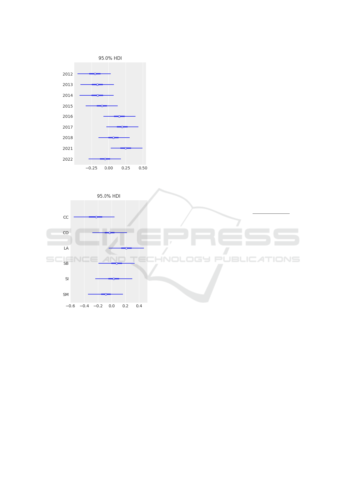
Figure 3: Random Effects of Academic Year on Freshmen

Attrition Log-Odds.

Figure 4: Random Effects of School on Freshmen Attrition

Log-Odds.

there is non-negligible ﬂuctuation. The 95%HDI =[-

0.221347,0.200628], which also suggests a mixed

scenario. The forest plot (see Figure 4) shows the

variability of log-odds of freshmen attrition across all

six schools.

Some schools, such as the School of Computer

Science & Mathematics (CC), have mostly negative

log-odds values, which point to a lower likelihood

of students dropping out in or after their freshman

year. Instead, freshmen students belonging or as-

signed to the School of Liberal Arts (LA) -and Be-

havioral Sciences (SB) to a much lesser extent- have

a higher likelihood of leaving the institution. To quan-

tify this difference, with a median log-odds value of

-0.25 for CC and 0.2 for LA, the odds ratio between

LA and CC is e

0.2

−0.25

= 1.57, which means that

LA freshmen are 1.57 times more likely to drop out

than CC freshmen. These results underscore the need

for additional analysis and potential targeted retention

strategies: while Computer Science & Mathematics

seems to be more sheltered from freshmen attrition

concerns, the positive log-odds exhibited by Liberal

Arts (LA) and, to some extent, Behavioral Sciences

(SB) may require that the institution dig deeper into

the underlying causes of these attrition rate values.

To answer RQ3 (Bayesian vs frequentist hierar-

chical models) we ran a frequentist mixed effects

model (see Equation 3) with the same ﬁxed effects

predictors and group level intercepts for academic

year and school.

logit = b

+ b

AcademicYear

+ b

School

∑

j=1

AcademicYear

∼ Normal(0, σ

AcademicYear

)

School

∼ Normal(0, σ

School

)

p =

1 + exp(−logit)

(3)

We used pymer4 (Jolly, 2018), a Python library

that provides an interface to lme4, the popular R

GLMM package. The Pymer4 model produced simi-

lar signiﬁcant logistic regression coefﬁcients, validat-

ing the results in the Bayesian model, but there were

some important differences:

EffectiveGPA, isDeansList, Gender, UnmetNeed,

isCampusWorkStudy, and HasLoans remain strong

predictors in both models.

HSGPA, DistanceFromHome and PellAmount are

statistically signiﬁcant in both the frequentist and

the Bayesian models, but the Bayesian model out-

puts a very high overlap of the 95%HDI with ROPE

(91.765%, 100%, and 61.006% respectively), which

suggests limited practical impact.

The TutoringClassCount estimate is highly unsta-

ble in the Pymer4 model with a mean=-5.744 and

95% CI=(-105.501, 94.014). Instead, the Bayesian

model shrinks the estimate to a more reasonable

value: mean =-1.802, 95%HDI=(-2.732, -0.990).

This is important for dealing with small sample sizes

within some academic years and schools.

The frequentist intercept estimate has also a

very high variance, with mean=-3.153 and 95%CI=(-

24.075,17.769). In comparison, the Bayesian model

shrinks the estimate to mean=-2.341, 95%HDI=(-

2.8963,-1.808), reﬂecting the true baseline dropout

rate much better.

The frequentist model gives a single estimate

and conﬁdence interval, assigning signiﬁcance based

Predictors of Freshmen Attrition: A Case Study of Bayesian Methods and Probabilistic Programming

129

Table 5: Summary of Frequentist Model Estimates.

Component Estimate SE 2.5% CI 97.5% CI OR OR 2.5% CI OR 97.5% CI Z-stat P-val Signiﬁcance

Intercept -3.153 10.675 -24.075 17.769 0.043 0.000 5.214e+07 -0.295 0.768

EFC 0.013 0.035 -0.056 0.083 1.013 0.946 1.086 0.376 0.707

EffectiveGPA -0.769 0.037 -0.841 -0.696 0.464 0.431 0.498 -20.854 0.000 ***

HSGPA 0.127 0.043 0.042 0.212 1.136 1.043 1.237 2.926 0.003 **

isDeansList [1.0] 0.573 0.096 0.385 0.761 1.774 1.470 2.140 5.985 0.000 ***

NumAPCourses -0.054 0.039 -0.130 0.022 0.947 0.878 1.022 -1.405 0.160

USCitizen [1.0] -0.281 0.204 -0.680 0.118 0.755 0.507 1.126 -1.379 0.168

UnmetNeed 0.370 0.044 0.285 0.456 1.448 1.330 1.577 8.507 0.000 ***

WaitListed [1.0] 0.113 0.116 -0.114 0.340 1.120 0.893 1.405 0.978 0.328

DistanceFromHome 0.124 0.028 0.069 0.179 1.132 1.072 1.196 4.431 0.000 ***

Gender [M] -0.240 0.076 -0.389 -0.091 0.787 0.678 0.913 -3.154 0.002 **

HasLoans [1.0] -0.211 0.077 -0.362 -0.060 0.810 0.697 0.942 -2.741 0.006 **

isCampusWorkStudy [1.0] -0.612 0.113 -0.833 -0.391 0.542 0.435 0.677 -5.425 0.000 ***

isDivisionI [1.0] -0.011 0.099 -0.206 0.184 0.989 0.814 1.202 -0.107 0.915

isFirstGeneration [1.0] 0.105 0.103 -0.097 0.306 1.110 0.907 1.358 1.016 0.310

PellAmount -0.180 0.040 -0.258 -0.102 0.835 0.773 0.903 -4.536 0.000 ***

StudentOfColor [1.0] 0.166 0.101 -0.033 0.365 1.180 0.968 1.440 1.635 0.102

TutoringClassCount -5.744 50.898 -105.501 94.014 0.003 0.000 6.756e+40 -0.113 0.910

Random Effects Academic Year: Var = 0.034, Std = 0.184 School: Var = 0.023, Std = 0.152

Evaluation metrics Log-likelihood: -3227.289 AIC: 6494.577

purely on p-values, whereas the Bayesian model gives

a full posterior distribution of the model parameters,

which helps in gauging uncertainty in regression co-

efﬁcients.

As for random effects, the frequentist model re-

ports variance and standard deviation for each group

(academic year and school), which makes it difﬁcult

to assess variability among groups when the group ef-

fects are small. Random effects in the Pymer4 model

are estimated independently. This means that each

group (academic year and school) gets its own sep-

arate estimated effect, without the effect being pulled

towards the mean, even if there are a small number

of observations per group. In contrast, the Bayesian

model reports the full posterior for each group, which

helps in detecting some signiﬁcant deviation, as ex-

plained in the above paragraphs (see RQ2, Figure 3,

and Figure 4). Additionally, in the Bayesian model,

group effects are not treated independently, with par-

tial pooling regularizing group effects.

5 CONCLUSION

The goal of this research work was to apply Bayesian

hierarchical regression methods to analyze freshmen

attrition. The paper provides a guideline on how to

conduct the analysis and report the results and ﬁnd-

ings in the context of Bayesian methods and proba-

bilistic programming. The Bayesian framework is a

robust yet highly underutilized data-driven method-

ology in the academic analytics literature, especially

regarding student academic performance and attrition

analysis. The results presented in this paper identify

college academic performance, ﬁnancial need, gen-

der, tutoring, and work-study program participation as

having a signiﬁcant effect on the likelihood of fresh-

men attrition. The study showed ﬂuctuations across

time and schools that deserve deeper investigation and

potential customized intervention strategies. Also, a

comparison was made with an equivalent frequentist

mixed-effects model to highlight the differences be-

tween both approaches. The motivation of this re-

search is not only to provide a guideline on the use

of Bayesian methods for freshmen retention but also

to serve as a proof of concept that encourages other

researchers and practitioners to apply the Bayesian

framework in this domain. The practical implica-

tions of this work go beyond the methodological ap-

proach presented on the use of Bayesian inference and

probabilistic programming for student attrition analy-

sis. We believe that the analysis provides actionable

ﬁndings to stakeholders, administrators, and decision-

makers in higher education.

ACKNOWLEDGEMENTS

The author would like to thank the members of the

Retention Committee at Marist University for very

fruitful discussions. Special thanks go to Dr. Duy

Nguyen -Associate Professor of Mathematics, for his

thorough review of the paper, and to Ed Presutti -

Director of Data Science and Analytics, and Haseeb

Arroon -Director of Institutional Data, Research, and

Planning, for their work on the student and academic

data warehouse from which the data for this project

was extracted.

REFERENCES

Abril-Pla, O., Andreani, V., Carroll, C., Dong, L., Fonnes-

beck, C. J., Kochurov, M., Kumar, R., Lao, J., Luh-

mann, C. C., Martin, O. A., Osthege, M., Vieira, R.,

Wiecki, T. V., and Zinkov, R. (2023). Pymc: a modern,

DATA 2025 - 14th International Conference on Data Science, Technology and Applications

130

and comprehensive probabilistic programming frame-

work in python. PeerJ Computer Science, 9:e1516.

Bertolini, R., Finch, S. J., and Nehm, R. H. (2023). An

application of bayesian inference to examine student

retention and attrition in the stem classroom. Frontiers

in Education, 8:1073829.

Blei, D. M., Kucukelbir, A., and McAuliffe, J. D.

(2017). Variational inference: A review for statisti-

cians. Journal of the American Statistical Association,

112(518):859–877.

Campbell, J. P. (2007). Utilizing Student Data Within

the Course Management System to Determine Under-

graduate Student Academic Success: An Exploratory

Study. Doctoral dissertation, Purdue University, West

Lafayette, IN. UMI No. 3287222.

Capretto, T., Piho, C., Kumar, R., Westfall, J., Yarkoni, T.,

and Martin, O. A. (2022). Bambi: A simple interface

for ﬁtting bayesian linear models in python.

Carpenter, B., Gelman, A., Hoffman, M. D., Lee, D.,

Goodrich, B., Betancourt, M., Brubaker, M., Guo, J.,

Li, P., and Riddell, A. (2017). Stan: A probabilistic

programming language. Journal of Statistical Soft-

ware, 76(1):1–32.

Chen, X., Zou, D., and Xie, H. (2022). A decade of learning

analytics: Structural topic modeling based bibliomet-

ric analysis. Education and Information Technologies,

27:10517–10561.

Dai, M., Hung, J., Du, X., Tang, H., and Li, H. (2021).

Knowledge tracing: A review of available technolo-

gies. Journal of Educational Technology Development

and Exchange (JETDE), 14(2):1–20.

Deberard, S. M., Julka, G. I., and Deana, L. (2004). Pre-

dictors of academic achievement and retention among

college freshmen: A longitudinal study. College Stu-

dent Journal, 38(1):66–81.

Delen, D. (2010). A comparative analysis of machine learn-

ing techniques for student retention management. De-

cision Support Systems, 49(4):498–506.

Duane, S., Kennedy, A. D., Pendleton, B. J., and Roweth,

D. (1987). Hybrid monte carlo. Physics Letters B,

195(2):216–222.

Easystats (2024). Highest density interval (hdi). Accessed:

2024-08-18.

Gelman, A. and Hill, J. (2006). Data Analysis Using Re-

gression and Multilevel/Hierarchical Models. Cam-

bridge University Press, Cambridge.

Gelman, A., Hill, J., McCarty, C. B., Dunson, D. B., Ve-

htari, A., and Rubin, D. B. (2013). Bayesian Data

Analysis. Chapman and Hall/CRC, 3rd edition.

Gelman, A., Jakulin, A., Pittau, M. G., and Su, Y.-S. (2008).

A weakly informative default prior distribution for lo-

gistic and other regression models. The Annals of Ap-

plied Statistics, 2(4):1360 – 1383.

Geman, S. and Geman, D. (1984). Stochastic relaxation,

gibbs distributions, and the bayesian restoration of im-

ages. IEEE Transactions on Pattern Analysis and Ma-

chine Intelligence, 6(6):721–741.

Gilks, W. R., Thomas, A., and Spiegelhalter, D. J. (1994).

A language and program for complex bayesian mod-

elling. The Statistician, 43:169–178.

Greenland, S., Senn, S. J., Rothman, K. J., Carlin, J. B.,

Poole, C., Goodman, S. N., and Altman, D. G. (2016).

Statistical tests, p values, conﬁdence intervals, and

power: a guide to misinterpretations. European jour-

nal of epidemiology, 31(4):337–350.

Hastings, W. K. (1970). Monte Carlo sampling methods us-

ing Markov chains and their applications. Biometrika,

57(1):97–109.

Homan, M. D. and Gelman, A. (2014). The no-u-turn sam-

pler: adaptively setting path lengths in hamiltonian

monte carlo. J. Mach. Learn. Res., 15(1):1593–1623.

Jolly, P. (2018). Pymer4: Connecting r and python for linear

mixed modeling. Journal of Open Source Software,

3(31):862.

Kruschke, J. (2014). Doing Bayesian Data Analysis: A Tu-

torial with R, JAGS, and Stan. Academic Press.

Kruschke, J. K. (2018). Rejecting or accepting parame-

ter values in bayesian estimation. Advances in Meth-

ods and Practices in Psychological Science, 1(2):270–

280.

Kumar, R. et al. (2019). Arviz: A uniﬁed library for ex-

ploratory analysis of bayesian models in python. Jour-

nal of Open Source Software, 4(33):1143.

Laur

ıa, E., Stenton, E., and Presutti, E. (2020). Boosting

early detection of spring semester freshmen attrition:

A preliminary exploration. In Proceedings of the 12th

International Conference on Computer Supported Ed-

ucation - Volume 2: CSEDU, pages 130–138, ISBN

978-989-758-417-6, ISSN 2184-5026. SciTePress.

NCES (2022). Undergraduate retention and graduation

rates. Condition of education, National Center for Ed-

ucation Statistics, U.S. Department of Education, In-

stitute of Education Sciences. Retrieved August 2024.

NSCRC (2014). Completing college: A national view of

student attainment rates – fall 2014 cohort. Techni-

cal report, National Student Clearinghouse Research

Center.

Phan, D., Pradhan, N., and Jankowiak, M. (2019). Compos-

able effects for ﬂexible and accelerated probabilistic

programming in numpyro.

Plummer, M. (2003). Jags: A program for analysis of

bayesian graphical models using gibbs sampling. In

Proceedings of the 3rd International Workshop on

Distributed Statistical Computing (DSC 2003), pages

1–10, Vienna.

Vehtari, A., Gelman, A., and Gabry, J. (2017). Prac-

tical bayesian model evaluation using leave-one-out

cross-validation and waic. Statistical Computing,

27(2):1413–1432.

Watanabe, S. (2010). Asymptotic equivalence of bayes

cross validation and widely applicable information

criterion in singular learning theory. Journal of Ma-

chine Learning Research, 11:3571–3594.

Westfall, J. (2017). Statistical details of the default priors in

the bambi library.

Yudelson, M. V., Koedinger, K. R., and Gordon, G. J.

(2013). Individualized bayesian knowledge tracing

models. In Artiﬁcial Intelligence in Education, vol-

ume 7926 of Lecture Notes in Computer Science,

pages 171–180. Springer.

Predictors of Freshmen Attrition: A Case Study of Bayesian Methods and Probabilistic Programming

131