Behavior Detection of Quadruped Companion Robots Using CNN:

Towards Closer Human-Robot Cooperation

Piotr Artiemjew

1 a

, Karolina Krzykowska-Piotrowska

2 b

and Marek Piotrowski

3 c

Faculty of Mathematics and Computer Science, University of Warmia and Mazury in Olsztyn, Poland

Faculty of Transport, Warsaw University of Technology, Poland

Faculty of Economic Sciences, University of Warmia and Mazury in Olsztyn, Poland

Keywords:

Mobile Robotics, Behaviour Tracking, Convolutional Neural Networks (CNN), Spot Boston Dynamics,

Unitree Go2 Pro, Human–Robot Interaction.

Abstract:

In a world where mobile robotics is increasingly entering various areas of people’s lives, creating systems

that track the behavior of mobile robots is a natural step toward ensuring their proper functioning. This is

particularly important in cases where improper use or unpredictable behavior may pose a threat to the envi-

ronment and, above all, to humans. It should be emphasized that this is especially relevant in the context of

using robotic solutions to improve the quality of life for people with special needs, as well as in human–robot

interaction. Our primary aim was to verify the experimental effectiveness of classiﬁcation based on convo-

lutional neural networks for detecting behaviours of four-legged robots. The study focused on evaluating the

performance in recognising typical robot poses. The research was conducted in our robotics laboratory, using

Spot and Unitree Go2 Pro quadruped robots as experimental platforms. We addressed the challenging task of

pose recognition without relying on motion tracking — a difﬁculty particularly pronounced when dealing with

rotations.

1 INTRODUCTION

With increasing automation and the growing imple-

mentation of robots in our daily lives, it is becoming

crucial to develop effective systems to recognise

their behaviour, especially in the context of walking

robots that are designed to act as human companions.

The coexistence of human and machine poses new

challenges, and one of the most important is to under-

stand and predict the actions of robots to ensure the

safety and comfort of their human companions. The

research problem related to human-robot cooperation

has been one of the important research threads un-

dertaken in various ﬁelds of science for years. There

is no shortage of research initiatives regarding the

cooperation of speciﬁc social groups with robots, for

example older people and people with reduced mobil-

ity (Hersh(2015); Harmo(2005); Kawamura(1994);

Jackson(1993); Martinez-Martin(2020)).

https://orcid.org/0000-0001-5508-9856

https://orcid.org/0000-0002-1253-3125

https://orcid.org/0000-0002-1977-5995

It is worth emphasizing that there is a notice-

able need for interdisciplinary research on this issue

and the need to implement deep learning technology

to improve human-robot cooperation. In this context,

creating advanced systems to recognise the behaviour

of walking robots is essential to build trust and

harmonious coexistence between humans and their

mechanical companions. These systems enable the

identiﬁcation and interpretation of a range of robot

actions, which is key to ensuring their effective and

safe interaction with humans and the environment

(Krzykowska(2021)). By understanding the inten-

tions and capabilities of robots, it becomes possible

not only to avoid potential misunderstandings and

conﬂicts, but also to better exploit their potential to

help humans. Furthermore, the development of such

systems is not only of practical importance, but also

ethical. As robots become more autonomous and

capable of making decisions, it becomes important

that their actions are transparent and understandable

to humans. This, in turn, raises the issue of account-

ability and control of machines, which is essential

to maintain public trust in the face of the growing

presence of robots in our lives. Consequently, the

Artiemjew, P., Krzykowska-Piotrowska, K. and Piotrowski, M.

Behavior Detection of Quadruped Companion Robots Using CNN: Towards Closer Human-Robot Cooperation.

DOI: 10.5220/0013548200003964

In Proceedings of the 20th International Conference on Software Technologies (ICSOFT 2025), pages 281-287

ISBN: 978-989-758-757-3; ISSN: 2184-2833

281

development of effective systems for recognising the

behaviour of walking robots is not only a technolog-

ical challenge, but also a social imperative to ensure

that advances in robotics serve the good of humanity

by promoting supportive and positive relationships

between humans and their robotic companions. The

use of deep machine learning methods in the context

of potentially improving the effectiveness of human-

robot cooperation is a popular research thread. This

applies, for example, to learning emotion expressions

to a human companion robot (Churamani(2017)),

deep learning of emotion and sentiment recognition

(Fung(2016)) or a gesture recognition approach for

facilitating interaction between humans and robots

(Yahaya(2019)). Our main objective was to design

a classiﬁer that gives the ability to distinguish the

position of a companion robot. To this end, we cre-

ated a collection of samples in the robotics laboratory

representing the different classes. As a reference

classiﬁer, we used convolutional neural networks,

a classical LeNet type (Lecun(1998); Goodfel-

low(2016); Almakky(2019)) and a quaternion neural

network (Niemczynowicz(2023)).

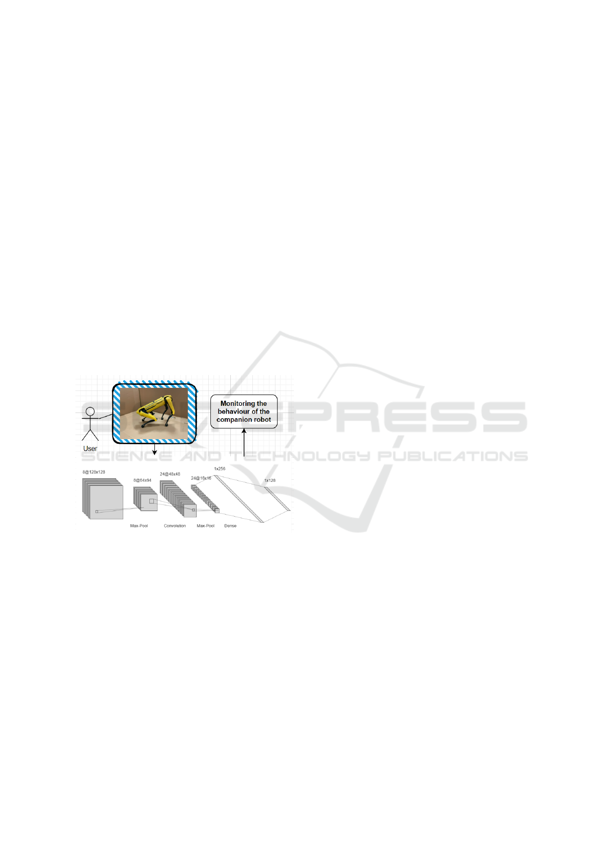
Figure 1: Graphical abstract.

The structure of the paper is as follows: Section

2 and Section 3 present potential applications and re-

lated work. Section 4 describes the model settings.

Section 5 introduces the experimental setup and sum-

marizes the results. Finally, Section 6 provides the

conclusions. Let’s move on to discuss the research

methodology.

2 POTENTIAL APPLICATIONS

Although the primary objective of this study was

to experimentally evaluate the effectiveness of robot

pose classiﬁcation using convolutional and quaternion

neural networks, the developed approach holds sig-

niﬁcant potential for broader application in various

domains. Below, we outline several promising areas

where such methods could be further explored and

adapted for real-world use.

2.1 Assistive Technologies and Elderly

Care

Behaviour recognition systems can be implemented

in robotic assistants used by elderly or mobility-

impaired individuals. These systems may help detect

abnormal robot behaviours, such as falls or movement

errors, improving user safety and enabling timely in-

tervention by caregivers or autonomous correction

mechanisms.

2.2 Industrial Automation and Logistics

In warehouses and production lines, legged or mo-

bile robots are becoming more common. Recognising

robot posture in such settings can support task moni-

toring, reduce collision risks, and improve system di-

agnostics by detecting mechanical anomalies through

motion patterns.

2.3 Search and Rescue Operations

In disaster response scenarios—such as building col-

lapses or hazardous environments—legged robots are

deployed for terrain exploration. The ability to recog-

nise and interpret the robot’s posture could inform op-

erators about potential failures or obstacles, aiding in

faster and safer decision-making during search and

rescue missions.

2.4 Forestry and Agroforestry

This area represents an underresearched but promis-

ing domain for mobile robotics. Robots equipped

with pose recognition can assist in tasks such as mon-

itoring forest conditions, navigating uneven terrain, or

performing semi-autonomous actions. The approach

may support enhanced motion control, safety, and en-

vironmental awareness (Schraick(2024)).

2.5 Educational Robotics and Social

Interaction

In educational or public engagement settings, robots

are used to interact with children or general audi-

ences. Recognising robot positions may improve

the naturalness and responsiveness of these interac-

tions—for example, by allowing the robot to sit, ob-

ICSOFT 2025 - 20th International Conference on Software Technologies

282

serve, or mimic human gestures in a socially appro-

priate manner.

2.6 Competitive Robotic Sports

In robotic competitions such as RoboCup, posture

recognition may contribute to real-time game analy-

sis, rule enforcement, and performance diagnostics.

Detecting intentional or faulty movement patterns

could aid in improving training algorithms and tac-

tical planning.

2.7 Public Space Patrol and

Surveillance

Mobile robots used in campus security, parks, or pub-

lic infrastructure could beneﬁt from autonomous be-

haviour monitoring. Posture recognition could assist

in detecting anomalies—such as falling, obstruction,

or route deviation—and trigger alerts for human su-

pervision or corrective actions.

2.8 Rehabilitation and Physical

Therapy

Robots used in therapeutic exercises may require the

ability to adapt to patient movements. Recognising

their own posture in relation to patients can enhance

interactive protocols and allow for more dynamic and

personalised rehabilitation sessions.

3 RELATED WORKS

Traditional approaches based on handcrafted fea-

tures and rule-based logic are still commonly used

in robotic systems but show limited adaptability in

complex scenarios. As discussed by Fabisch et al.

(Fabisch(2019)), the application of machine learning

to behavior learning in robotics, especially for legged

or sensor-rich robots, remains an evolving ﬁeld with

signiﬁcant potential and outstanding challenges. In

contrast, deep learning methods, particularly convo-

lutional neural networks (CNNs), offer signiﬁcant ad-

vantages in terms of feature extraction and scalability

(Ruiz(2018); Cebollada(2022)). These methods have

been successfully applied in activity recognition do-

mains, such as human behaviour classiﬁcation, and

are gaining relevance in robotic applications involv-

ing visual input. Moreover, in the context of social

robotics, understanding robot posture plays an impor-

tant role in building trust and engagement during hu-

man–robot interaction.

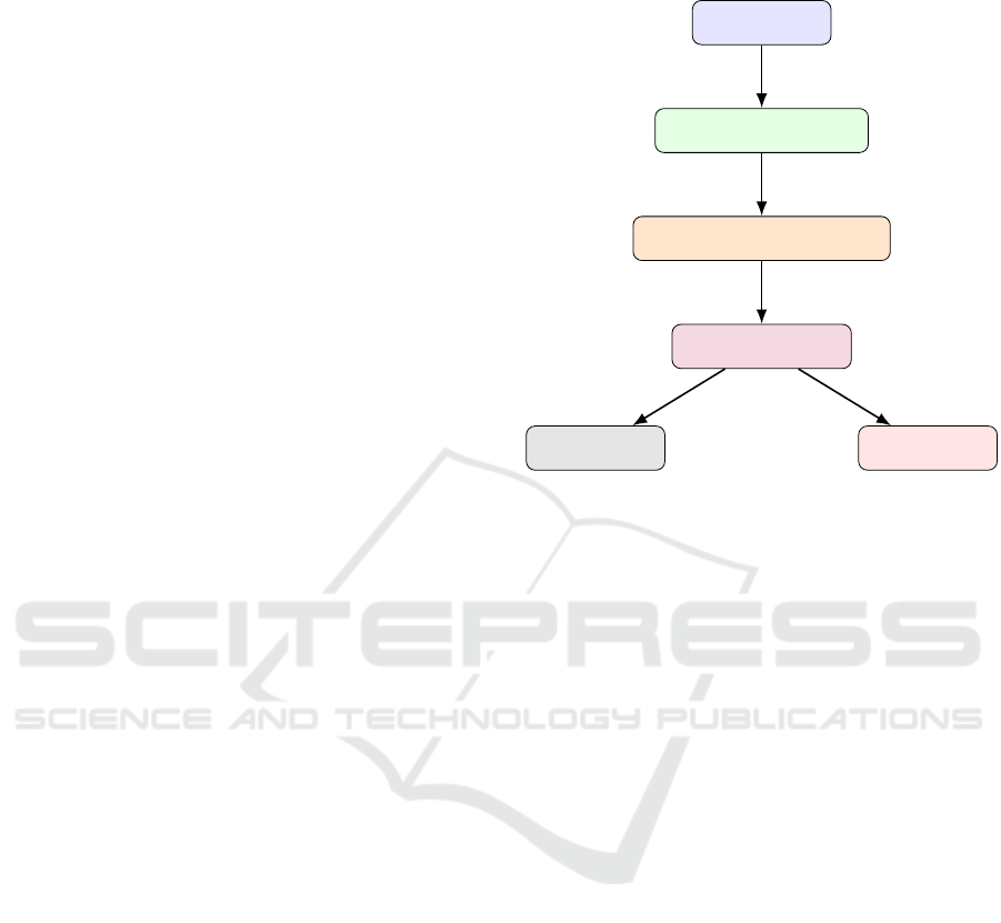
4 METHODOLOGY

Camera / Sensor

Image Capture & Preprocessing

Behavior Recognition (Trained Model)

Detected Behavior & Pose

User Interface

Safety Center

Figure 2: System architecture for quadruped robot behavior

recognition.

Our primary aim was to verify the experimental effec-

tiveness of classiﬁcation based on convolutional neu-

ral networks on four-legged robots behaviour detec-

tion - using Spot and Unitree Go2 pro. LeNet (Le-

cun(1998); Goodfellow(2016); Almakky(2019)) type

ConvNet (Goodfellow(2016); Lou(2020)) - see the

Fig. 3. And we tested the effectiveness of a quater-

nion neural network (Niemczynowicz(2023)), whose

architecture you can see in Fig. 4.

model_real = kr.Sequential([

layers.Conv2D(8, kernel_size=(3, 3), activation="relu",

input_shape=Xtr.shape[1:]),

layers.MaxPooling2D(pool_size=(2, 2)),

layers.Conv2D(16, kernel_size=(3, 3), activation="relu"),

layers.MaxPooling2D(pool_size=(2, 2)),

layers.Conv2D(16, kernel_size=(3, 3), activation="relu"),

layers.MaxPooling2D(pool_size=(2, 2)),

layers.Conv2D(32, kernel_size=(3, 3), activation="relu"),

layers.MaxPooling2D(pool_size=(2, 2)),

layers.Flatten(),

layers.Dropout(0.5),

layers.Dense(1, activation=None)

])

model_real.compile(optimizer=’adam’,

loss=kr.losses.BinaryCrossentropy(from_logits=True),

metrics=[kr.metrics.BinaryAccuracy(threshold=0.0)])

Figure 3: Applied architecture in ConvNet.

Let’s move on to discuss the experimental part and

the results of the study.

Behavior Detection of Quadruped Companion Robots Using CNN: Towards Closer Human-Robot Cooperation

283

model_hyper = kr.Sequential(

[

layers.Input(shape=Xtr.shape[1:]),

HyperConv2D(2, kernel_size=(3, 3), activation="relu", algebra = quat),

layers.MaxPooling2D(pool_size=(2, 2)),

HyperConv2D(4, kernel_size=(3, 3), activation="relu", algebra = quat),

layers.MaxPooling2D(pool_size=(2, 2)),

HyperConv2D(4, kernel_size=(3, 3), activation="relu", algebra = quat),

layers.MaxPooling2D(pool_size=(2, 2)),

HyperConv2D(8, kernel_size=(3, 3), activation="relu", algebra = quat),

layers.MaxPooling2D(pool_size=(2, 2)),

layers.Flatten(),

layers.Dropout(0.5),

layers.Dense(1, activation=None),

]

)

quat = np.array([[-1,+1,-1],[-1,-1,1],[1,-1,-1]])

Figure 4: Applied architecture of Qwaternion network. quat

= Quaterions.

5 EXPERIMENTAL PART AND

RESULTS

In the deep neural network classiﬁcation experiments,

we divided the image sets into a training subset and

the validation test set with an 60/40 split. To es-

timate the quality of the classiﬁcation, we used the

Monte Carlo Cross Validation (Xu(2001); Goodfel-

low(2016)) technique (MCCV5, i.e., ﬁve times train

and test), presenting average results. In the exper-

iments, the test (validation) system is applied in a

given iteration to the model to check the ﬁnal efﬁ-

ciency and observe the overlearning level. By eval-

uating in each iteration of learning an independent

validation set (not affecting the network’s learning

process), we can determine the degree of generaliza-

tion of the model. In evaluating experiments, accu-

racy in a balanced version is often recommended, i.e.,

the average accuracy of all classes classiﬁed (Broder-

sen(2010)). In our experiments, we use the Coss En-

tropy Loss version, which can exceed a value of 1, to

clearly indicate where the model is malfunctioning.

We scaled images to 100 × 100 pixels to ensure the

same size of the input for the network. We fed the ar-

tiﬁcial neural network with data after four alternating

convolutional and max-pooling steps. We used max-

pooling because it is the most effective technique for

reducing the sizes of images, which works well with

neural network models. Such an approach turned out

to be better in practice than average pooling (Brown-

lee(2019)). The convolutional layers extract features

from images before they are fed into the network. The

activation function of hidden layers was ReLU, and

the output layer had raw values. The loss function

took the form of categorical cross-entropy. Thus, it

could be higher than one. To train the neural network,

we used RGB color channels and applied the Adam

optimizer (Kingma(2015)). For quaternion networks,

we used the HSV color model. We carried out the

training over 50 epochs (for Spot), and 100 epochs

(for Unitree). The batch size was 16. We ﬁtted the

above parameters experimentally.

In the experimental session we learned to distin-

guish spot behaviour (and for the most challengig

poses also Unitree Go2 pro poses), we have a full list

of experimental variations in Tab 1. We can see sam-

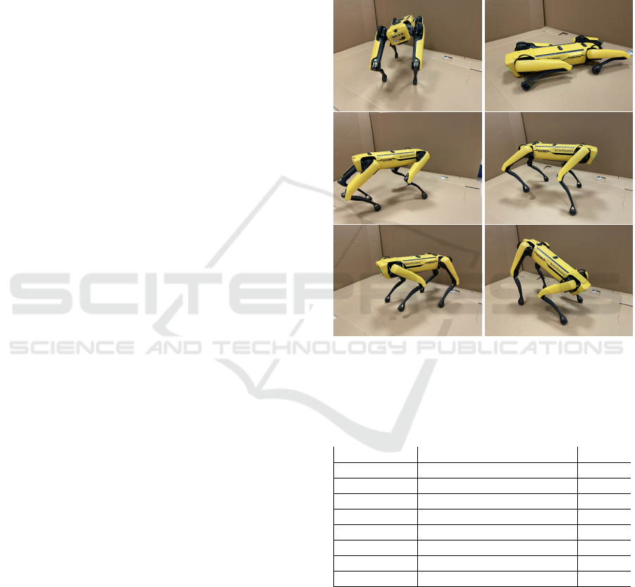
ples of each class in Fig 5.

Figure 5: Examples of Spot poses: Top left = Rotation on

the shorter side, Top right = Sitting, Middle left = Standing,

Middle right = Turning left, Bottom left = Turning right,

Bottom right = Rotation on the longer side.

Table 1: Experimental variants.

Pose

Result

Spot case

Standing Sitting robot Fig. 6

Standing Rotation on the longer side Fig. 7

Standing Rotation on the shorter side Fig. 8

Turning left Turning right Fig. 9

Standing Turning right Fig. 10

Unitree case

Turning left Turning right Fig. 12

We performed all the experiments in a similar

way. Thus, our results show how the MCCV5 method

works in each learning epoch and present the results

of ﬁve internal tests and the average result.

Various poses of the robot were analyzed, includ-

ing standing vs. sitting, standing vs. turning on the

long side, standing vs. turning on the shorter side,

turning left vs. turning right, and standing vs. turning

ICSOFT 2025 - 20th International Conference on Software Technologies

284

right, which are described in detail and shown in Fig-

ures 6, 7, 8, 9, 10 and 12 and listed in Table 1. Exper-

imental results showed that the quaternion network,

thanks to the use of faster and more compact convo-

lution, learns faster than the classical convolutional

network, but the ﬁnal results of the two networks are

similar.

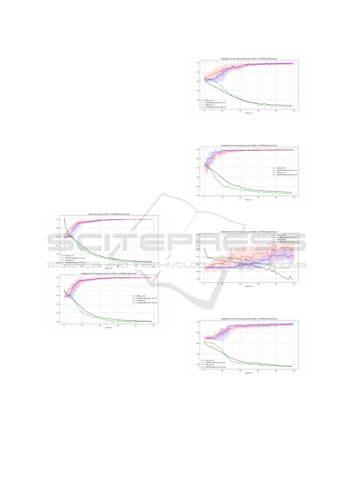
The following results were achieved in the differ-

ent variants of the robot’s posture recognition:

In the standing vs sitting variant, results close to

100% were achieved for the validation data, allowing

the learning to stop after only about 30 iterations. In

the variant of standing vs rotating on the longer and

shorter side, the results exceeded 95% for the valida-

tion data, also after about 30 iterations. Recognizing

the direction of rotation (left vs. right) proved to be

the most difﬁcult, with results exceeding 80% after

about 50 iterations. In this case, the quaternion net-

work showed better performance. In the variant of

standing vs. turning right, the results exceeded 90%,

with a slight advantage for ConvNet in the more difﬁ-

cult variant.

Figure 6: Spot case study: Classiﬁcation using CNNs and

QCNNs. Standing vs sitting robot. The top image shows

the learning process, the bottom validation.

Seeing the results of the study, we decided to test

the most difﬁcult variant, the recognition between

turning right and left on another four-legged robot

Unitree Go2 pro - see samples of classes 11. We can

conclude that the quaternion network learns faster and

achieves more stable results although comparable to

the CNN. When recognising poses on which we see

a left or right turn, our models achieved an average

accuracy efﬁciency of around 0.75. That is, slightly

worse results than detection when observing Spot.

Figure 7: Spot case study: Classiﬁcation using CNNs and

QCNNs. Standing vs Rotation on the longer side. Valida-

tion of the learning process.

Figure 8: Spot case study: Classiﬁcation using CNNs and

QCNNs. Standing vs Rotation on the shorter side. Valida-

tion of the learning process.

Figure 9: Spot case study: Classiﬁcation using CNNs and

QCNNs. Turning right vs left. Validation of the learning

process.

Figure 10: Spot case study: classiﬁcation using CNNs and

QCNNs. Standing vs Turning right. Validation of the learn-

ing process.

Behavior Detection of Quadruped Companion Robots Using CNN: Towards Closer Human-Robot Cooperation

285

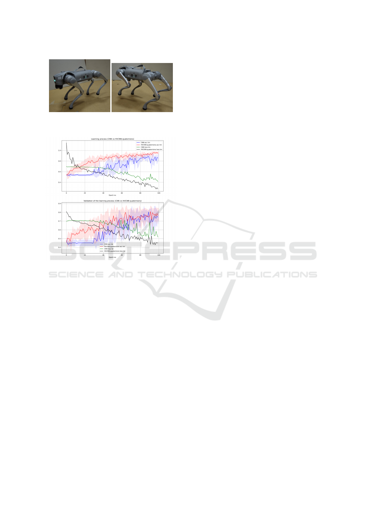
Figure 11: Examples of Unitree Go2 pro robot poses: Top

= Turning left, Bottom = Turning right.

Figure 12: Unitree Go2 pro case study: classiﬁcation using

CNNs and QCNNs. Turning right vs left. The top image

shows the learning process, the bottom validation.

6 CONCLUSIONS

The research showed that the use of a Quaternion

Neural Network and a classical Convolutional Net-

work (ConvNet) type of LeNet is an effective method

for learning and recognizing the behavior of a walk-

ing companion robot, such as the Spot robot from

Boston Dynamics and Unitree Go2 pro. Experimental

results conﬁrmed the high performance of both types

of networks in different variants of the robot’s behav-

ior recognition, with slight differences in performance

depending on the task’s complexity. The imperfection

of the technological solutions and the dependence of

the level of effectiveness of their operation on many

external factors may pose some kind of threat to their

users and the environment. In this context, the devel-

opment of systems monitoring the behavior of walk-

ing robots used to cooperate with humans seems to

be a necessity. The results of our study have impor-

tant implications for the development of robot behav-

ior detection and recognition systems, which can help

improve robot-human interaction and increase the ef-

ﬁciency of robots in a variety of environments. We

believe that this may be extremely important, espe-

cially in the context of cooperation between walking

robots and people with special needs, including the

elderly and disabled people. In future research, we

plan to add an additional motion tracking module to

support robot behaviour detection.

ACKNOWLEDGEMENTS

We would like to thank Aleksandra Szpakowska for

preparing the data for the experiments. The article

has been supported by the Polish National Agency

for Academic Exchange Strategic Partnership Pro-

gramme under Grant No. BPI/PST/2021/1/00031.

Research was funded by the Warsaw University of

Technology within the Excellence Initiative: Re-

search University (IDUB) programme Young PW.

HELPER – High Expert Level optimization of the

Process of Exploitation of a companion Robot dedi-

cated for elderly No.1820/103/Z01/2023. This work

has been supported by a grant from the Ministry of

Science and Higher Education of the Republic of

Poland under project number 23.610.007-110.

REFERENCES

LeNail, A. NN-SVG: Publication-Ready Neural Network

Architecture Schematics. J. Open Source Softw. 2019,

4, 747.

Lecun, Y.; Bottou, L.; Bengio, Y.; Haffner, P. Gradient-

based learning applied to document recognition. Pro-

ceedings of the IEEE 1998, 86(11), 2278–2324.

Lou, G.; Shi, H. Face image recognition based on convolu-

tional neural network. China Communications 2020,

17(2), 117–124.

Hunter, J. D. Matplotlib: A 2D Graphics Environment.

Computing in Science Engineering 2007, 9(3), 90–95.

Brownlee, J. A Gentle Introduction to Deep Learning for

Face Recognition. Deep Learning for Computer Vi-

sion 2019.

Kingma, D. P.; Ba, J. Adam: A Method for Stochastic Op-

timization. CoRR 2015, abs/1412.6980.

Qing-Song Xu and Yi-Zeng Liang, Monte Carlo cross

validation, Chemometrics and Intelligent Laboratory

Systems, vol. 56, no. 1, pp. 1–11, 2001. DOI:

10.1016/S0169-7439(00)00122-2.

Brodersen, K. H., Ong, C. S., Stephan, K. E., and Buh-

mann, J. M.: The Balanced Accuracy and Its Posterior

Distribution, in Proceedings of the 2010 20th Interna-

tional Conference on Pattern Recognition (ICPR ’10),

IEEE Computer Society, USA, 2010, pp. 3121–3124,

https://doi.org/10.1109/ICPR.2010.764

ICSOFT 2025 - 20th International Conference on Software Technologies

286

Almakky, I.; Palade, V.; Ruiz-Garcia, A. Deep Convolu-

tional Neural Networks for Text Localisation in Fig-

ures From Biomedical Literature. In Proceedings of

the 2019 International Joint Conference on Neural

Networks (IJCNN); 2019; pp. 1–5.

Goodfellow, I.; Bengio, Y.; Courville, A. Deep Learn-

ing. MIT Press, 2016. Available online: http://www.

deeplearningbook.org (accessed on 4 March 2023).

Niemczynowicz, A., Kycia, R. A., Jaworski, M.,

Siemaszko, A., Calabuig, J. M., Garcia-Rafﬁ, L.

M., Schneider, B., Berseghyan, D., Perﬁljeva, I.,

Nov

ak, V., Artiemjew, P.: Selected aspects of com-

plex, hypercomplex and fuzzy neural networks. CoRR

abs/2301.00007 (2023)

Hersh, M. Overcoming barriers and increasing indepen-

dence–service robots for elderly and disabled people.

International Journal of Advanced Robotic Systems,

2015, 12.8: 114.

Harmo, P., et al. Needs and solutions-home automation

and service robots for the elderly and disabled. In:

2005 IEEE/RSJ international conference on intelli-

gent robots and systems. IEEE, 2005. p. 3201-3206.

Kawamura, K.; Iskarous, M. Trends in service robots for the

disabled and the elderly. In: Proceedings of IEEE/RSJ

International Conference on Intelligent Robots and

Systems (IROS’94). IEEE, 1994. p. 1647-1654.

Jackson, R. D. Robotics and its role in helping disabled peo-

ple. Engineering Science & Education Journal, 1993,

2.6: 267-272.

Martinez-Martin, E.; Escalona, F.; Cazorla, M. Socially as-

sistive robots for older adults and people with autism:

An overview. Electronics, 2020, 9.2: 367.

Churamani, N., et al. Teaching emotion expressions to a hu-

man companion robot using deep neural architectures.

In: 2017 international joint conference on neural net-

works (IJCNN). IEEE, 2017. p. 627-634.

Fung, P., et al. Towards empathetic human-robot interac-

tions. In: Computational Linguistics and Intelligent

Text Processing: 17th International Conference, CI-

CLing 2016, Konya, Turkey, April 3–9, 2016, Re-

vised Selected Papers, Part II 17. Springer Interna-

tional Publishing, 2018. p. 173-193.

Yahaya, S. W., et al. Gesture recognition intermediary

robot for abnormality detection in human activities.

In: 2019 IEEE Symposium Series on Computational

Intelligence (SSCI). IEEE, 2019. p. 1415-1421.

Krzykowska-Piotrowska, K.; Dudek, E.; Siergiejczyk, M.;

Rosi

nski, A.; Wawrzy

nski, W. Is Secure Communica-

tion in the R2I (Robot-to-Infrastructure) Model Pos-

sible? Identiﬁcation of Threats. Energies 2021, 14,

4702. https://doi.org/10.3390/en14154702

Schraick, L.-M. (2024). Usability in Human-Robot Collab-

orative Workspaces. Universal Access in the Informa-

tion Society (UAIS), https://doi.org/10.1007/s10209-

024-01163-6

Ruiz-del-Solar, J., Loncomilla, P. and Soto, N.: A Survey

on Deep Learning Methods for Robot Vision, arXiv

preprint arXiv:1803.10862, 2018.

Fabisch, A., Petzoldt, C., Otto, M., and Kirchner, F.: A Sur-

vey of Behavior Learning Applications in Robotics

– State of the Art and Perspectives, arXiv preprint

arXiv:1906.01868, 2019.

Cebollada, S. Pay

a, L., Jiang, X. and Reinoso, O.: Devel-

opment and use of a convolutional neural network for

hierarchical appearance-based localization,” Artiﬁcial

Intelligence Review, vol. 55, no. 4, pp. 2847–2874,

2022. 10.1007/s10462-021-10076-2.

Behavior Detection of Quadruped Companion Robots Using CNN: Towards Closer Human-Robot Cooperation

287