
Parameter Transfers for Warm-Started QAOA
Julian Obst
a
, Felix Truger
b
, Johanna Barzen
c
and Frank Leymann
d
Institute of Architecture of Application Systems, University of Stuttgart, Universit
¨
atsstraße 38, Stuttgart, Germany
Keywords:
Quantum Approximate Optimization Algorithm, Warm-Start.
Abstract:
Variational Quantum Algorithms (VQAs) run shallow parameterized quantum circuits on quantum devices and
are thus suitable for current limited hardware. However, adverse effects like barren plateaus and local optima
may hinder the classical parameter optimization. Warm-starting techniques attempt to alleviate such problems
by utilizing pre-computed approximations or known solutions to initialize VQAs. In this work, we analyze a
combination of two different kinds of warm-starts, based on biased initial states and parameter transfers, re-
spectively. In particular, we investigate a warm-started variant of the Quantum Approximate Optimization Al-
gorithm (WS-QAOA) applied to the MAXCUT problem and analyze the transferability of optimized parameter
values between random graphs. We leverage their decomposition into subgraphs and regularities among these
subgraphs to facilitate parameter transfers for WS-QAOA and demonstrate a transfer for a random graph.
1 INTRODUCTION
Quantum computing is an emerging field in com-
puter science with promising applications in various
domains, such as chemistry and optimization (Cao
et al., 2018; Harrigan et al., 2021). However, this
potential cannot be fully realized yet, as current
Noisy Intermediate-Scale Quantum (NISQ) devices
are error-prone and the size of quantum circuits that
can be executed successfully is limited (Preskill,
2018; Leymann and Barzen, 2020). Errors can accu-
mulate during lengthy computations on quantum de-
vices, making circuit depth a particular issue. Thus,
circuits executed on current hardware should be shal-
low. Until fault-tolerant quantum computers become
available, Variational Quantum Algorithms (VQAs)
bridge the gap and make use of current, limited quan-
tum hardware (Cerezo et al., 2021).
VQAs resort to shallow parameterized quan-
tum circuits, frequently referred to as Ans
¨
atze,
that are executed on the quantum computer, while
their parameters are adjusted by an optimizer that
is executed on classical hardware. A prominent
example of such algorithms is the Quantum Approx-
imate Optimization Algorithm (QAOA) (Farhi et al.,
2014), which is designed to solve various combi-
a
https://orcid.org/0000-0002-1898-2167
b
https://orcid.org/0000-0001-6587-6431
c
https://orcid.org/0000-0001-8397-7973
d
https://orcid.org/0000-0002-9123-259X
natorial optimization problems like the MAXCUT,
MINIMUMVERTEXCOVER, and TRAVELINGSALES-
PERSON problem (Farhi et al., 2014; Zhang et al.,
2022; Ruan et al., 2020).
However, VQAs may run into problems like
barren plateaus and local minima (Wang et al., 2021;
Bittel and Kliesch, 2021), which are detrimental
effects in the optimization that may lead to slow con-
vergence of the algorithm. One class of approaches
that tries to circumvent these problems and speed
up the computation are so-called warm-starts (Egger
et al., 2021; Galda et al., 2021; Truger et al., 2024a).
The general idea is to give the algorithm an advantage
by utilizing known or efficiently generated results,
such as optimized parameter values from related
problem instances and classically approximated
parameterizations or solutions for the problem at
hand. Several techniques can be used to warm-start
quantum algorithms (Truger et al., 2024a). In
particular, there are two major groups of approaches
for warm-starting VQAs. The first group encodes an
approximate solution into the algorithm itself. In this
sense, Egger et al. propose a QAOA variant called
warm-started QAOA (WS-QAOA) for the MAXCUT
problem, that uses an approximate solution to prepare
a biased initial state and improve upon the approx-
imation (Egger et al., 2021). Similarly, Tate et al.
propose a biased initial state directly based on a re-
laxation of MAXCUT to warm-start the QAOA (Tate
et al., 2023). The second group focuses on obtaining
Obst, J., Truger, F., Barzen, J., Leymann and F.
Parameter Transfers for Warm-Started QAOA.
DOI: 10.5220/0013539300004525
In Proceedings of the 1st International Conference on Quantum Software (IQSOFT 2025), pages 37-48
ISBN: 978-989-758-761-0
Copyright © 2025 by Paper published under CC license (CC BY-NC-ND 4.0)
37

good initial parameter values that are improved upon
in the optimization. One way to get good parameter
values is to identify similar problem instances and
use their optimized parameters for another instance.
This transfer of parameters has been investigated,
e.g., by Galda et al. for QAOA (Galda et al., 2021).
This work combines the two approaches and in-
vestigates the possibility of parameter transfers be-
tween instances of the MAXCUT problem for Egger
et al.’s WS-QAOA. Therefore, we analyze the algo-
rithm’s performance on subgraphs of random graphs
up to degree 5 to explore regularities and a structure
for potential parameter transfers. Moreover, we de-
scribe how the insights gained from this analysis are
utilized to determine good parameter values for larger
graphs when warm-starting is employed. We demon-
strate this by finding good initial parameter values for
a 50-node random graph instance with a maximum
degree of 5 that are very close to the actual optimum.
The remaining sections of this paper are organized
as follows. Section 2 introduces the necessary back-
ground and related work. Section 3 describes how the
investigation was performed. The insights and results
as well as their utilization are covered in Section 4.
Section 5 discusses limitations and possible extension
of the method. Finally, Section 6 summarizes our
work and gives an outlook on possible future work.
2 BACKGROUND AND RELATED
WORK
The QAOA, one of the most prominent examples
of VQAs, was introduced in a seminal work by
Farhi et al. (2014). They illustrate that the algorithm
can be applied to approximate solutions to the MAX-
CUT problem. In short, the parameterized circuit that
is executed on the quantum computer consists of an
initialization to a uniform superposition and two sub-
circuits parameterized by
ˆ
γ and
ˆ
β, respectively. These
subcircuits are referred to as the problem circuit and
mixer. The problem circuit is constructed such that
its ground state is an optimal solution to the problem
at hand, while the mixer’s ground state is the initial
state of the overall circuit. The problem circuit and
mixer are repeated p times, which is referred to as
the QAOA depth of the Ansatz. Thus, the overall cir-
cuit implements a trotterized approximation of an adi-
abatic evolution that aims to achieve a transition from
the known ground state of the mixer into the unknown
ground state of the problem circuit, representing an
optimal solution. The algorithm converges towards
an optimum with the increase of the QAOA depth p.
A partitioning of the nodes of an undirected graph
into two sets is called a cut, with the number of edges
between the two sets being the value of the cut. A
MAXCUT or Maximum Cut is thus a partitioning that
maximizes the number of edges between the two sets.
In the case of weighted graphs, the goal is to maxi-
mize the sum of the edge weights between both sets.
The problem is well known to be NP-hard, but can
be approximated. Executing the QAOA for a set of
parameters creates a distribution of cuts, with the ex-
pected value of the cut being referred to as the energy.
The objective of the QAOA is to optimize this energy,
thereby producing good cuts.
Egger et al. (2021) adapted the QAOA to uti-
lize approximations to the MAXCUT problem as
a starting point by encoding them into the initial
state of the quantum circuit. The adaptation, called
Warm-Started QAOA (WS-QAOA), makes use of the
best known classical approximation algorithm for
the MAXCUT problem by Goemans and Williamson
(1995). Thereby the QAOA is enhanced in the sense
that less optimization may be necessary if the ini-
tial state is biased towards a good solution as a start-
ing point or, conversely, lower QAOA depth suf-
fices to reach a good result quality, making WS-
QAOA a promising algorithm for current NISQ hard-
ware. Specifically, instead of the uniform superpo-
sition, each qubit in the initial state of WS-QAOA
is more likely to be in either of the states |0⟩ or |1⟩
as prescribed by the approximation obtained from the
Goemans-Williamson algorithm (GW). The deviation
of the initial state from the uniform superposition and
the bias towards the approximation is controlled by a
regularization parameter ε. In addition, the mixer in
WS-QAOA is adapted for the modified initial state.
Egger et al. also propose a modified mixer that does
not have the initial state as a ground state, however, as
a first step we focus on the version that is in line with
the adiabatic evolution behind QAOA.
Another way to warm-start VQAs, is by finding
a good initialization for the Ansatz parameters, e.g.,
by pre-computing viable parameter values or transfer-
ring optimized parameters from related problem in-
stances (Truger et al., 2024a). The advantage here
is, that all VQAs can be warm-started by parameter
initializations without having to change the underly-
ing algorithm. The difficulty lies in finding viable pa-
rameter values that yield good results. One approach
is to optimize parameters for a smaller problem in-
stance and then transferring the optimized parame-
ter values to the actual target problem. To this end,
Galda et al. (2021) investigated the transfer of opti-
mal QAOA parameter values for the MAXCUT prob-
lem between problem instances. In particular, they
IQSOFT 2025 - 1st International Conference on Quantum Software
38

considered regular and random graphs up to a degree
of 8 and 6, respectively. This analysis showed that a
transfer between instances is possible and primarily
depends on the degree of subgraphs. For instance, a
transfer between k- and d-regular instances is likely
to be successful, provided that k and d are both even
or both odd. Our work extends this analysis to WS-
QAOA, for which the degree alone is not enough to
guarantee a successful transfer anymore.
There are several works similar to the ones intro-
duced above. Tate et al. (2023) successfully warm-
start the QAOA for MAXCUT with low-rank Burer-
Monteiro relaxations, while Cain et al. (2022) show
that a warm-start that naively initializes the circuit
with an approximation fails. Shaydulin et al. (2021)
introduce a repository for optimized QAOA parame-
ters that enables parameter transfers. Brandao et al.
(2018) show that the landscapes of large 3-regular
graphs are instance independent, whereas Akshay
et al. (2021) demonstrated a concentration of opti-
mal QAOA parameters for p ∈ {1, 2}. Shaydulin
et al. (2023) explain how to transfer parameters for
weighted MAXCUT. More generally, Truger et al.
(2024b) document warm-starting patterns for quan-
tum algorithms, including warm-starts via biased ini-
tial states and warm-starts via parameter transfers.
However, none of the work that we are aware of com-
bines a warm-start via a biased initial state with a pa-
rameter transfer.
The Quantum Modelling Extension (QuantME)
introduces a warm-starting task that conceptually
facilitates parameter transfers for WS-QAOA in
workflow-based quantum applications (Beisel et al.,
2023). In particular, this task provides configuration
attributes for warm-starting quantum executions uti-
lizing biased initial states and parameter initializa-
tions. However, it does not provide guidance on how
to effectively combine the two.
3 PARAMETER TRANSFER FOR
WS-QAOA
This section introduces our approach to parameter
transfers for WS-QAOA for the MAXCUT problem.
We first give an overview of the decomposition of
such parameter transfers based on subgraphs, before
we provide more details on the concrete experimental
setup for our analysis.
3.1 Overview
On a high level, our approach considers the transfer-
ability of parameters for subgraphs to derive a param-
eter transfer for a targeted problem instance. As was
shown in the original QAOA paper, the energy values
for a particular graph can be evaluated as the sum over
subgraph contributions (Farhi et al., 2014). We inves-
tigate the QAOA at p = 1, where only two parameters
need to be optimized. To expand the investigation to
p > 1 one must conduct the analysis on larger and
more subgraphs as will be discussed in Section 5. In
general, the investigation is centered around energy
landscapes of subgraphs. Energy landscapes are cre-
ated by systematically evaluating the QAOA circuit in
its parameter space and computing the corresponding
energy values. They allow for the comparison of en-
ergy extrema within the parameter space to draw con-
clusions about the transferability of parameter values.
To determine the transferability of parameters for
WS-QAOA, we investigate the energy landscapes for
different subgraphs while considering different possi-
ble initial states. Specifically, we assess whether op-
timal parameter values coincide, i.e., whether good
values for one instance are also suitable for another.
For our purposes, optimal parameters are located at
maxima, since we investigate the MAXCUT problem.
For a fixed set of parameters, the energy is evaluated
according to Equation (1) (cf. Galda et al. (2021)).
⟨C⟩
|
ˆ
γ,
ˆ
β⟩
= ⟨
ˆ
γ,
ˆ
β|C |
ˆ
γ,
ˆ
β⟩
= ⟨
ˆ
γ,
ˆ
β|
1
2
∑
(i, j)∈E
(1−Z
i
Z
j
)|
ˆ
γ,
ˆ
β⟩
=
|E|
2
−
1
2
∑
(i, j)∈E
⟨
ˆ
γ,
ˆ
β|Z
i
Z
j
|
ˆ
γ,
ˆ
β⟩
=
|E|
2
−
1
2
∑
(i, j)∈E
e
i j
(
ˆ
γ,
ˆ
β)
(1)
C in Equation (1) is the problem-specific operator in
QAOA and e
i j
is the contribution of an individual
edge in the set of edges E. This means, instead of
looking at the graph as a whole, we can break down
the problem by investigating how each edge influ-
ences the energy. The contribution e
i j
can be deter-
mined by looking at the subgraph that is induced by
the edge. The induced subgraph consists of the edge
itself, called the central edge that connects the central
nodes, and all nodes (and connecting edges) that are
at most distance p away. Therefore, the worst case is
that we have to consider as many subgraphs, as there
are edges in a graph. In reality, however, many sub-
graphs appear repeatedly. For example, for k-regular
graphs, there are k different subgraphs that need to be
investigated. Additionally, in WS-QAOA we need to
consider different initializations due to different pos-
sible approximations encoded into the initial state as
Parameter Transfers for Warm-Started QAOA
39

warm-starts. Thus, the number of energy landscapes
that need to be taken into account increases in the con-
text of WS-QAOA compared to standard QAOA.
To facilitate the identification of individual sub-
graphs we introduce the following notation, which is
adapted from Galda et al. (2021): A subgraph is re-
ferred to as (x-y)-z, where x ≤y are the number of
neighbors of the two central nodes and z is the num-
ber of neighbors shared by both nodes. For example,
the graph in Figure 1 is called (3-3)-0.
3.2 Experimental Setup
Assuming a fixed configuration of WS-QAOA, our
analysis extends over every possible initialization for
every subgraph of regular graphs up to degree 5. After
accounting for isomorphisms, this yields 214 different
landscapes. Expanding the scope of the investigation
to random graphs up to degree 5 yields 35 subgraphs
and increases the total number of landscapes to 620.
For reasons discussed in Section 4.2, this number can
be reduced to 558.
To create landscapes for a subgraph, one first
needs to construct the QAOA circuit, where each node
corresponds to one qubit. As discussed previously, we
adopt WS-QAOA from Egger et al. (2021) in its ba-
sic form. The first consideration is the depth p that
we choose as p = 1 resulting in a circuit with two pa-
rameters (γ, β) to be optimized and two-dimensional
energy landscapes that can be illustrated. Addition-
ally, WS-QAOA can be adjusted by its regulariza-
tion parameter ε ∈ [0,0.5], where ε = 0.5 leads to the
original QAOA and lower values increase the influ-
ence of the approximate solution utilized as a warm-
start. To put more emphasis on the warm-start, we
choose ε = 0.1. To prepare the biased initial state,
a rotation R
Y
by an angle θ
i
is applied to each qubit
q
i
, where θ
i
= 2arcsin
√
ε if the corresponding node
is initialized with 0, and θ
i
= 2arcsin
√
1−ε if it is
initialized with 1. Thus, a single qubit reproduces
its initialization with probability 1 −ε if we were to
measure it. For example, a qubit of a node initial-
ized with 0 measures |0⟩ with probability 1 −ε. An
example for the WS-QAOA circuit is given in Fig-
ure 1. After constructing the circuit, it is executed
on a simulator where we measure the qubits of the
central edge, which are q
0
,q
1
in all our experiments.
The portion of measurements, where q
0
̸= q
1
is the
probability of the edge being cut, i.e., the energy con-
tribution e
i j
of Equation (1). We create the land-
scape by sampling the energy in the parameters space
(γ,β) ∈[0, 2π] ×[0, π]. To this end, we sample 30 pa-
rameter values for each dimension to obtain the two
sets Γ and B, resulting in a total of |Γ| ·|B| = 900
equidistant samples. Since we are dealing with un-
weighted graphs, the landscapes are periodic, and it
is sufficient to analyze the parameter space within the
given range.
4 RESULTS
This section presents the results of the analysis for
subgraphs and the transferability of parameters be-
tween graphs in WS-QAOA for MAXCUT. In partic-
ular, we first look at the landscapes of regular graphs,
before moving on to random graphs. Next, we intro-
duce a transferability map to analyze the transferabil-
ity in more detail. Finally, we utilize the insights to
find good parameters for a larger graph instance. For
verification and reproducibility, the results can be ac-
cessed online (Obst and Truger, 2024). This includes
a visualization of all subgraphs with their correspond-
ing landscapes and numeric data.
q
0
:
R
Y
(2.5)
•
ZZ(-γ)
• •
R
Y
(-2.5) R
Z
(2β) R
Y
(2.5)
q
1
:
R
Y
(0.6)
•
ZZ(-γ)
• •
R
Y
(-0.6) R
Z
(2β) R
Y
(0.6)
q
2
:
R
Y
(0.6)
•
ZZ(-γ)
R
Y
(-0.6) R
Z
(2β) R
Y
(0.6)
q
3
:
R
Y
(2.5)
ZZ(-γ)
•
R
Y
(-2.5) R
Z
(2β) R
Y
(2.5)
q
4
:
R
Y
(0.6)
•
ZZ(-γ)
R
Y
(-0.6) R
Z
(2β) R
Y
(0.6)
q
5
:
R
Y
(0.6)
•
R
Y
(-0.6) R
Z
(2β) R
Y
(0.6)
Figure 1: Example subgraph and its circuit consisting of initialization, problem circuit, and mixer separated by dashed lines.
The subgraph is depicted with its initialization where purple and yellow nodes correspond to an initialization of 0 and 1
respectively. Each qubit corresponds to one node of the graph, where the first two qubits q
0
,q
1
are the central nodes, and each
ZZ gate corresponds to an edge in the graph. Since ε = 0.1, the parameters of the initial R
Y
gates are 2arcsin
√
ε ≈ 0.64 if
the initialization of the corresponding node is 0, and 2arcsin
√
1−ε ≈ 2.50 if the initialization is 1. The parameter values are
rounded to one decimal place.
IQSOFT 2025 - 1st International Conference on Quantum Software
40
0
π
2
π
0
π
2π
0
π
2
π
0
π
2π
0
π
2
π
0
π
2π
0
π
2
π
0
π
2π
0
π
2
π
0
π
2π
0
π
2
π
0
π
2π
0
π
2
π
0
π
2π
0
π
2
π
0
π
2π
0
π
2
π
0
π
2π
0
π
2
π
0
π
2π
0
π
2
π
0
π
2π
0
π
2
π
0
π
2π
low high
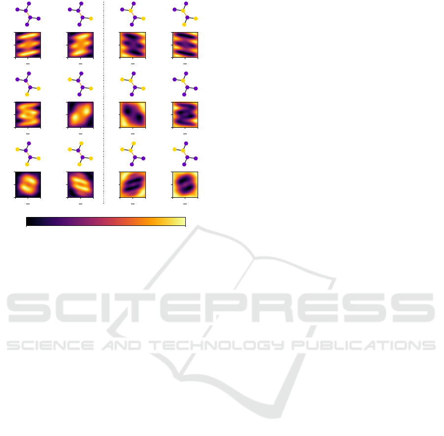
Figure 2: Graph (3-3)-0, one of the three subgraphs of a 3-
regluar graph, with all its initializations up to isomorphism.
An initialization with 0 is represented by a purple node, an
initialization with 1 by a yellow node. The central edge that
is being measured is highlighted. Values of the landscape
are normalized, as we only care about maxima and minima,
not their exact value. The graphs are ordered such that all
initializations on the left have central nodes that are initial-
ized equally. Additionally, the landscapes are paired with
their mirrored version on the opposite side.
4.1 Landscapes for Regular Graphs
In the following, we analyze landscapes for regular
graphs and describe regularities found between the
landscapes.
4.1.1 3-Regular Graphs
Examining the landscapes for subgraphs on their own
helps us gain a better understanding of the reasons for
good transferability and identify regularities among
the results. First, we focus on the subgraphs of regular
graphs, as their regularities also appear in other sub-
graphs. Figure 2 shows the most general subgraph in
the sense that there are no common neighbors among
the nodes of the central edge. The graph is depicted
with every possible initialization indicated by a color
coding: Nodes initialized to 0 are colored in purple,
nodes initialized to 1 are colored in yellow. Isomor-
phisms are not shown, as they produce identical re-
sults. Moreover, we also consider it an isomorphism
if all initializations of the nodes are inverted, as such
configurations would also result in the same energy
values. When checking for isomorphisms, it is im-
portant to label the central edge, as it is the one be-
ing measured as described in Section 3.2. This makes
no difference for d-regular graphs with d ≥ 3, but is
relevant for small random graphs. That way, all 12
different initializations and their corresponding land-
scapes are presented in Figure 2. All landscapes are
normalized for the visualization. The maximum is the
brightest spot and the minimum the darkest. For the
transfer of parameters, the actual energy values are
less relevant than the locations of extrema, particu-
larly the global maxima, as these mark the optimal
parameter values. Therefore, we can disregard that
scale for transfers and in the visualizations. For a bet-
ter illustration of regularities among the landscapes,
they are grouped in two categories: The first (left) half
shows landscapes where outskirts have a low energy,
while the center generally shows a high energy. In the
second (right) half, it is the other way around. The
difference between the two groups lies in the initial-
ization of the central nodes. In the first category, the
nodes are initialized identically, i.e., the central edge
is not part of the cut. For the second category, the
edge is part of the cut, i.e., nodes are initialized dif-
ferently. Intuitively, this is explained by the fact that
we only look at the energy of the central edge. Given
a good initialization, parameters that favor the initial
state, i.e., parameters around zero, should be expected
to result in high energy values.
The chosen arrangement of Figure 2 highlights an-
other relationship between the landscapes. The six
landscapes on the right-hand side appear to be in-
verted mirror images of those on the left-hand side.
More precisely, the landscapes on the opposite side
have the same shape but appear to be flipped verti-
cally/horizontally and inverted, i.e., minima of one
landscape become maxima in the other and vice versa.
Landscapes that are related this way also have a con-
nection in the respective graphs: Taking one of the
central nodes and inverting the initialization of each
adjacent node, including the other central node, re-
sults in an isomorphic graph. Future work may
provide a better understanding of this phenomenon
through a deeper mathematical analysis.
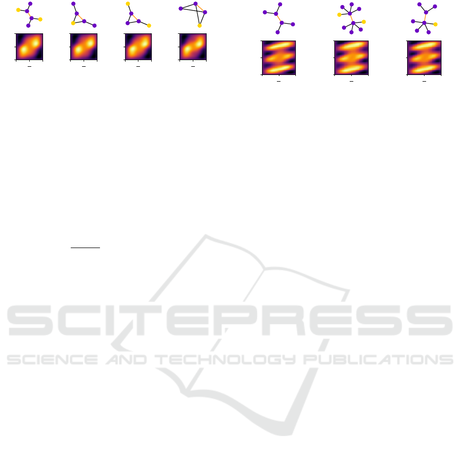
4.1.2 Subgraphs with Common Neighbors
As mentioned before, we can understand the sub-
graphs (x-y)-z with z ≥ 1 as a version of the
graph (x-y)-0 where the central nodes have z com-
mon neighbors. Analogous to the observations of
Galda et al. (2021), the landscapes of k-regular sub-
graphs are very similar for a fixed k when their ini-
tialization is equivalent, as explained in the follow-
ing. This fact is demonstrated in Figure 3 with equiv-
alent initializations for the subgraphs (3-3)-0, (3-3)-1,
Parameter Transfers for Warm-Started QAOA
41
0
π
2
π
0
π
2π
0
π
2
π
0
π
2π
0
π
2
π
0
π
2π
0
π
2
π
0
π
2π
Figure 3: Subgraphs of 3-regular graphs with similar land-
scapes. From left to right, the subgraphs are (3-3)-0, (3-
3)-1, (3-3)-1, (3-3)-2. Similar landscapes arise when identi-
cally initialized neighbors are merged into a common neigh-
bor of both central nodes. The MAD between the normal-
ized landscapes is at most 0.03. The second and third land-
scape look alike, because splitting the common neighbor
would result in isomorphic graphs.
and (3-3)-2, which induce resembling landscapes. To
quantify this similarity, we determine the Mean Ab-
solute Difference (MAD). For two normalized energy
landscapes E
1
,E
2
and sets of parameter values Γ, B it
is calculated as follows:
MAD(E
1
,E
2
) =
1
|Γ|·|B|
∑
(γ,β)∈Γ×B
|
E
1
(γ,β) −E
2
(γ,β)
|
Since the energy is in the interval [0, 1], identical land-
scapes have an MAD of 0 and opposite landscapes
have an MAD of 1. In Figure 3, the graph (3-3)-1
is shown twice with different initialization, yet their
landscapes look identical. To be precise, their MAD
is 0.02. While they are in fact non-isomorphic, the
similarity appears because of their relation to (3-3)-
0: In both cases, replacing the common neighbor of
the central nodes with two identically initialized sep-
arate nodes would create the same version of (3-3)-
0, i.e., the initialization of these subgraphs is equiva-
lent to the one depicted for (3-3)-0. Hence, (3-3)-0 is
the most general of the three subgraphs, as it allows
for the largest number of initializations, and “split-
ting” common neighbors by replacing them with sep-
arate nodes returns one of these instances. Since both
graphs are descendants of the same parent, we con-
sider only one of them in further analyses.
Increasing z, i.e., introducing common neighbors,
does not induce additional initializations to consider
over those known for the most general subgraph.
Conversely, there are initializations for (3-3)-0 for
which there is no equivalent initialization for (3-3)-1
or (3-3)-2. For example, in the top right graph de-
picted in Figure 2, the neighbors of the central nodes
are initialized both with 1 and both with 0, respec-
tively. Thus, no pair of these nodes could be merged
into a common neighbor and there is no equivalent
initialization for (3-3)-1.
0
π
2
π
0
π
2π
0
π
2
π
0
π
2π
0
π
2
π
0
π
2π
Figure 4: Different types of graphs that produce similar
landscapes. Neighbors that are initialized oppositely (one
is 0, the other is 1) cancel each other out. Removing them
does not substantially affect the landscape, i.e., the MAD
between them is smaller than 0.04.
4.1.3 Node Canceling
We briefly extend the analysis to subgraphs of
5-regular graphs, whose landscapes exhibit similari-
ties with those of 3-regular graphs. Namely, all land-
scapes of graph (3-3)-0 are also present among those
for (5-5)-0. An example is depicted in Figure 4.
Again, the similarity is due to a connection between
the underlying graphs: The central nodes of the (5-5)-
0 instance each have two neighbors that are initialized
differently. Disregarding such pairs of neighbors and
removing them from the graph on both sides of the
central edge results in the graph (3-3)-0 which pro-
duces the same landscape. In that sense, nodes can
cancel each other out and some initializations for (5-
5)-0 can be reduced to an equivalent initialization for
(3-3)-0. We refer to this as node canceling.
4.2 Random Graphs
The analysis can also be extended to random graphs.
In particular, the observations regarding common
neighbors and node canceling as introduced above
also apply to subgraphs of random graphs up to a
degree of 5. There are 35 subgraphs with a total
of 620 initializations. However, due to equivalent
initializations of graphs with common neighbors,
these can be reduced to 558 that need to be ana-
lyzed. For subgraphs of random graphs, the number
of neighbors of the central nodes can differ. For
example, the subgraph (3-5)-0 has a central node that
is missing two neighbors compared to (5-5)-0. The
rightmost example in Figure 4 illustrates that node
canceling also leads to resembling landscapes for
these types of subgraphs.
However, subgraphs of random graphs also intro-
duce landscapes with shapes that are not present for
regular graphs. Specifically, these landscapes appear
when the central nodes have a mixed parity, i.e., one
central node has an even and the other has an odd de-
gree. Still, subgraphs of random graphs exhibit the
IQSOFT 2025 - 1st International Conference on Quantum Software
42

same regularities as regular graphs, such as the mir-
rored relationship, merged nodes, and node cancel-
ing. Node cancelling is particularly interesting, as we
can also go in the opposite direction. Instead of re-
moving nodes, we can also add them to a graph, until
both central nodes have the same number of neigh-
bors. That way, subgraphs of random graphs can be
related to those of regular graphs. Clearly, this is only
possible if both central nodes have the same parity,
i.e., the degree of the central nodes is either even or
odd for both, as we add two nodes at a time. There-
fore, subgraphs of random graphs fall in one of two
categories: Either their central nodes have the same
parity, or they have mixed parity.
4.3 Transferability Map
This section examines the parameter transferability
between subgraphs of random graphs up to a degree
of 5 in more detail. To this end, we create a transfer-
ability map that visualizes the quality of such trans-
fers. We describe the construction of the transferabil-
ity map, the key observations, and the influence of the
degree of central nodes on the transferability.
4.3.1 Constructing the Transferability Map
To quantify the transferability between different sub-
graphs we determine a transferability coefficient τ. It
is calculated by taking the sampled optimal parame-
ters of one subgraph, the donor graph, and evaluating
their performance for another subgraph, the acceptor
graph. Determining the transferability is straightfor-
ward given the sampled landscapes. The transferabil-
ity coefficient τ can be computed as follows:
τ = avg
γ
max
,β
max
E
acc
(γ
max
,β
max
)
max
γ,β
{E
acc
(γ,β)}
(2)
We take the locations of global maxima in the sam-
pled landscape, (γ
max
,β
max
), of the donor subgraph
(there can be multiple maxima), evaluate the energy
E
acc
of the acceptor graph at these locations, normal-
ize by the maximum energy of the acceptor graph and
average the values. The coefficient τ is a value be-
tween 0 and 1, where 0 is the worst possible transfer-
ability and 1 is the optimal transferability.
Figure 5 shows the transferability coefficient for
every pair of two subgraphs and every initialization.
As Galda et al. noted, transferability is a directional
property. Therefore, the map is not symmetric along
its diagonal axis. The appearance of the map depends
on the arrangement of the subgraphs and their initial-
izations. While there are multiple possibilities to or-
der the graphs and their initializations, we decided for
an arrangement that is beneficial for the illustration of
some key observations. In particular, the graphs are
ordered by increasing minimum degree x and increas-
ing maximum degree y, i.e., first all the graphs (1-∗),
then (2-∗), etc. In addition, within each category, the
number of merged nodes z increases. The initializa-
tions of a single subgraph are divided into two groups,
the first having identically initialized central nodes,
the second having central nodes initialized oppositely.
The complete ordering of initializations of a subgraph
can be found online (Obst and Truger, 2024) together
with all landscapes.
4.3.2 Key Observations
As the transferability map contains a substantial
amount of information, we draw attention to key ob-
servations that unveil its utility. For one, the map
facilitates finding a suitable donor graph for a given
subgraph by scanning the respective row to identify
good candidates for a parameter transfer. Moreover,
the map helps to identify certain patterns and regular-
ities, to estimate the success of parameter transfers,
and to gain insights into properties that can be used to
make more general statements about transferability.
An important observation is, that the initialization
introduced with WS-QAOA significantly influences
the transferability. To be precise, the transferabili-
ties described by Galda et al. (2021) no longer apply
when a biased initial state is introduced, as these con-
ditions relied on graph structure alone. For example,
optimal parameters of a subgraph were trivially trans-
ferable to the same subgraph. However, for the same
instance in WS-QAOA with different initializations,
such transfers may fail. In particular, this is the case
across initializations where the central edge is cut and
others where the central edge is not cut, i.e., the two
groups described earlier. This restriction is visible in
the map by the fact that almost all subgraphs have
four distinct sectors that appear like a checkerboard
pattern (see Figure 5 box A). Note that such a section
contains all possible initializations for a single sub-
graph. The four sectors reflect all possible transfers
for the different initializations of the central nodes of
the donor and acceptor graph. They illustrate, that a
transfer is most successful, when the central nodes are
either initialized identically in both graphs or initial-
ized differently in both.
The next observation is, that the number of com-
mon neighbors has little influence on the transferabil-
ity (B), which is reflected in the similarity of sections
separated by dotted lines in Figure 5. This occurs be-
cause splitting common neighbors results in very sim-
ilar landscapes, as discussed above and shown in Fig-
ure 3. This phenomenon is already present when no
Parameter Transfers for Warm-Started QAOA
43
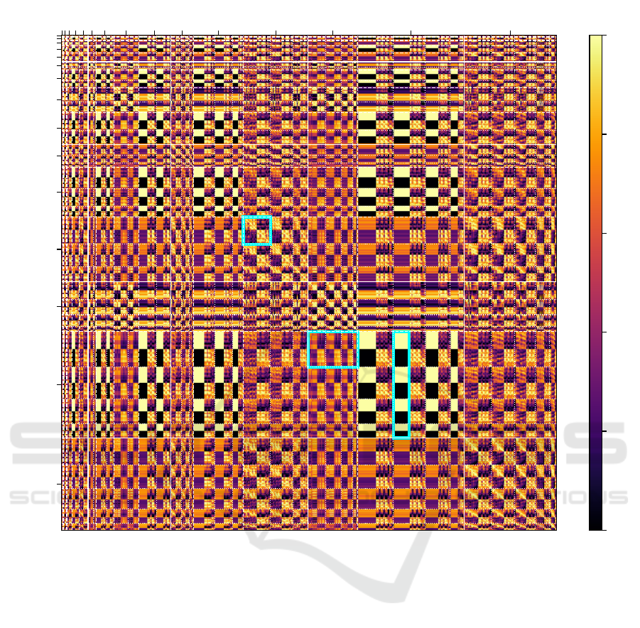
(1-∗) (2-∗) (3-3) (3-4) (3-5) (4-4) (4-5) (5-5)
Donor subgraph
(1-∗)
(2-2)
(2-3)
(2-4)
(2-5)
(3-3)
(3-4)
(3-5)
(4-4)
(4-5)
(5-5)
Acceptor subgraph
A B C
0.0
0.2
0.4
0.6
0.8
1.0
Transferability Coefficient
Figure 5: Transferability coefficients between every pair of subgraphs forming the Transferability Map. Each pixel is a
coefficient τ ∈ [0,1]. Dark colors indicate a bad transferability, bright colors indicate a good transferability. Each row is an
acceptor graph, each column a donor graph. Thick white lines distinguish graphs with differing minimum degree. Dashed
white lines separate graphs with different degrees of the central nodes, dotted lines further divide the number of common
neighbors. Overall, there are 35 subgraphs with a total of 558 initializations, starting with low degrees up to degree 5.
For clarity, some of the labels are omitted: (1-∗) stands for (1-1) through (1-5), (2-∗) stands for (2-2) through (2-5). The
highlighted sections and labels A, B, C serve as references for the observations described in Section 4.3.2.
biased initial state is involved (Galda et al., 2021). For
our purposes, this means that we need to prioritize the
initialization over the exact type of graph when look-
ing for a suitable donor graph.
Distinctive features of the map are absolutely per-
fect and disastrous transferabilities in some cases (C).
These become apparent as yellow and black patches
in Figure 5, most notably in the sections of (4-5).
Here we have optimal and worst case transferability
with coefficients of 1 and 0, respectively. This is due
to the shape of the respective landscapes, which ex-
hibit either exactly one maximum or one minimum
that is located right at the center of the landscape, re-
sulting in either a perfect transfer or the worst pos-
sible. Interestingly, these patches only appear for
donors whose central nodes are initialized the same.
However, the other sector, where the central nodes of
donor and acceptor are initialized oppositely, also ex-
hibits relatively high coefficients. This sector is par-
ticularly important for a parameter transfer of WS-
QAOA, as we will discuss in Section 4.4.
4.3.3 Influence of Node Degrees
Another important characteristic is the degree of the
central nodes, particularly, their parity. Galda et al. al-
ready described this and noted that a transfer between
IQSOFT 2025 - 1st International Conference on Quantum Software
44
k-regular and d-regular graphs is likely to be success-
ful, provided k and d are either both even or both odd
(Galda et al., 2021). When taking the initialization of
the central edge into account, this also seems to hold
with warm-starts in place. For example, (5-5) appears
to be a better donor for (3-3) than (4-4).
They also found that there is a good transfer-
ability between graphs ( j-k) and (l-m) provided that
{j, k, l, m} are all odd or all even. This also seems
true for WS-QAOA. For example, (3-5) as an accep-
tor has brighter sections when receiving parameters
from (5-5) rather than (4-4). Conversely, a transfer
from odd to even parity is also unlikely to be success-
ful. Notably, for (4-4) as an acceptor, the graph (2-4)
appears to be a better donor than (3-3). Interestingly,
graphs with even degrees do not show a checkerboard
pattern when receiving parameters from mixed parity
donors. An example for this would be (4-4) accepting
parameters from (4-5).
Moreover, Galda et al. showed cases of good
transferability between subgraphs with mixed parity.
With WS-QAOA, there seems to be good transferabil-
ity if both donor and acceptor graph have a mixed par-
ity, since the aforementioned sections with yellow and
black patches appear in exactly these cases.
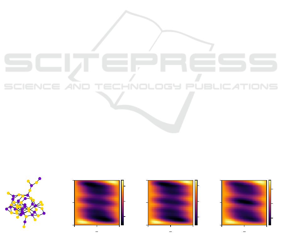
4.4 Application for Transferability
This section describes, how we can use the above
insights to obtain viable parameter values for larger
graphs composed of subgraphs. To this end, we de-
compose a larger graph into its subgraphs and try to
reduce the number of subgraphs that we have to con-
sider. We illustrate this application by determining vi-
able parameter values for the 50-node random graph
with 75 edges and a maximum degree of 5 shown in
Figure 6. A suitable initialization for the MAXCUT
problem on this graph was determined using the GW
algorithm (Goemans and Williamson, 1995).
The following procedure is based on the fact, that
the total energy is composed of contributions of the
subgraphs as described in Section 3.1. We can lever-
age the insights described above to obtain an approx-
imation of the landscape of the target graph shown in
Figure 6, from which we can derive a good parame-
terization. Specifically, subgraphs can be transformed
into a standardized format to increase the number of
isomorphic subgraphs, thereby reducing the number
of subgraphs that need to be considered and minimiz-
ing the effort required to determine good parameter
values. The first simplification is to consider only
subgraphs of the form (x-y)-0 by splitting common
neighbors of the central nodes. Since the landscapes
are very similar before and after the split, we do not
lose much information. Further, a graph falls in one
of three categories: Both central nodes have even
degrees, both have odd degrees or their degrees are
mixed. To transform these subgraphs further, we can
utilize the node canceling effects, i.e., add and remove
nodes that cancel out. In case that both central nodes
have even degrees, we can add two oppositely initial-
ized nodes at a time to a central node until the graph
takes the form of (4-4). If their degrees are odd, we
can add as many pairs as necessary to end up with (5-
5), and for mixed parity we can transform them into
instances of (4-5). In total, these 3 graphs allow for
90 different initializations.
Adding up the energy values of the subgraphs
with the respective initializations for each sampled
point results in the true energy landscape of the tar-
get graph. This true energy landscape is illustrated on
the left-hand side of Figure 6. Transforming the sub-
graphs before applying this procedure generates the
approximate landscape next to it. The target graph
consists of 38 different subgraphs, with the 3 most
frequent appearing 8, 7, and 5 times, respectively.
The simplifying transformations halve the number of
different subgraphs to 19, with the 3 most frequent
ones appearing 11, 10, and 9 times, respectively.
These 3 most frequent subgraphs produce the land-
scape shown on the right-hand side of Figure 6.
0
π
2
π
0
π
2π
True Energy
0
π
2
π
0
π
2π
Approximate Energy
0
π
2
π
0
π
2π
Energy of Top 3
40
50
60
40
50
60
15
20
25
Figure 6: Approximating the landscape of the graph on the left. The 50-node graph is pictured with its initialization, calculated
by the GW algorithm. Landscapes from left to right are the true energy landscape, its approximation after transforming all the
subgraphs to an equivalent of the form (4-4), (4-5), or (5-5), and the approximation of the landscape by only considering the
3 most frequent graphs after the simplifying transformations.
Parameter Transfers for Warm-Started QAOA
45

As a first observation, the landscapes show low
energy values in the center and high energy values
near the edges. Thus, they fall into the second group
of landscapes, where the central edge is cut (cf. Sec-
tion 4.1.1). This is expected because the initialization
is derived from a good approximation utilized for the
warm-start, resulting in subgraphs where many cen-
tral edges are already cut, i.e., initialized oppositely.
Further, it is expected that most of the subgraphs will
have many such edges, similar to the top right graph
of Figure 2. Therefore, the overall landscape resem-
bles the landscape of these subgraphs. Thus, an even
simpler transfer would be taking optimized parame-
ters from one of these graphs.
Evidently, the landscapes of Figure 6 appear very
similar despite the simplifications described above. In
particular, the MAD of true and approximate energy
is smaller than 0.02. If we consider only the three
most frequent graphs, the landscape changes notice-
ably, but not substantially. Since we only considered
the energy of 30 subgraphs for the latter, the total en-
ergy values are generally lower than in the original
landscape. However, it is not the total energy value
that is crucial for obtaining good parameter values
as mentioned in Section 4.1.1, but rather the location
of the maxima, that need to remain close. Keep in
mind, that the parameters (γ, β) were sampled in the
range of [0,2π] ×[0,π] with 30 samples per dimen-
sion. For the first approximation, the maximizing pa-
rameters are off by only one sample in the direction
of β, i.e., we are off by
π
30
from the sampled maxi-
mum. Surprisingly, the second approximation from
the top three subgraphs retains the maximum at the
exact same sample position as the true energy.
What the experiments have shown is, that we may
only focus our attention towards subgraphs that have
a central edge that is cut, as these are the most fre-
quent ones. Additionally, it can suffice to consider
only three types of graphs, one for each of the cate-
gories of even, odd, and mixed parity.
5 DISCUSSION AND
LIMITATIONS
While we analyzed many different subgraphs, and
demonstrated how to successfully transfer parame-
ters, there still remain open questions. Here, we dis-
cuss limitations of our study and how these shortcom-
ings may be addressed.
For one, it is not always feasible to calculate
the entire landscape, e.g., when larger QAOA depths
p > 1 are involved. In such cases, it is beneficial to re-
sort to the simplifications introduced above, identify
the most frequent subgraphs and optimize the energy
of their central edges. The parameter values can then
be used as an initialization for the instance at hand.
We suspect, that there is a concentration of good pa-
rameters in proximity to the optimal parameters of our
example. However, further research is required to ver-
ify whether this is the case.
As mentioned in Section 3.2, the choice of ε = 0.1
puts more emphasis on the initialization. However,
this parameter can also be selected differently or even
optimized, depending on the objective function in
use (Truger et al., 2022). Such alternative objective
functions for WS-QAOA may lead to different re-
sults for the landscapes and regularities for parameter
transferability.
The number of possible initializations grows
rapidly with the size of the graph. For this reason, we
only analyzed graphs up to degree 5, which may be
sufficient for some use cases. While we suspect that
the regularities described above generalize to larger
degrees, it is unclear whether they actually hold. It
would be interesting to see the transferability in WS-
QAOA for graphs up to degree 8 as analyzed by Galda
et al. Since many of their findings for standard QAOA
are consistent with ours for WS-QAOA, we suspect
that the regularities also hold for degrees up to 8.
However, an analysis could provide further insights
into the impact of the degree on transferability.
To calculate the transferability coefficient, we
sampled landscapes, which are limited to the grid of
points that were evaluated. Therefore, there may be
even better parameterizations than those correspond-
ing to the maxima in the sampled landscapes, which
could be obtained by additional optimization. Nev-
ertheless, the sampled landscapes appear smooth and
thus sufficient for the analysis of parameter transfers.
As noted above, our analysis is centered on a
QAOA depth of p = 1. While we suspect that some of
the regularities may also be present for p > 1 and that
techniques for determining good parameters could
still be applied, further study is required for confir-
mation. Such an investigation would involve larger
subgraphs, since edges that are distance p away from
the central edge form the subgraph and contribute to
its energy. This implies that more types of subgraphs
need to be analyzed, and more initializations have to
be considered. The rapid growth of initializations that
comes with increasing subgraph size may render an
analysis as thorough as for p = 1 impractical. More
than two circuit parameters further complicate an in-
vestigation, requiring the sampling of significantly
more data points and limiting the visualization.
Thus far, our analysis is limited to unweighted
graphs. Investigating weighted graphs requires a dif-
IQSOFT 2025 - 1st International Conference on Quantum Software
46

ferent approach, as the enumeration of every subgraph
is impossible with weights. Previous work explored a
transfer of QAOA parameters for the MAXCUT prob-
lem on weighted graphs (Shaydulin et al., 2023). It is
unclear how weighted graphs affect the transferability
of optimal parameters for WS-QAOA.
Our analysis was conducted based on noise-
less quantum simulation, however, using error-prone
NISQ hardware may pose additional challenges and
potentials for the approach of parameter transfers in
(WS-)QAOA. In particular, it was shown that apply-
ing the circuit cutting concept to QAOA for MAX-
CUT by breaking down the graph at hand can sig-
nificantly reduce the effects of noise on NISQ de-
vices (Bechtold et al., 2023). Circuit cutting focuses
on partitioning circuits into multiple smaller circuits,
whose individual execution results are post-processed
to obtain the original circuit’s result. On a higher
level, the approach of parameter transfers for WS-
QAOA based on subgraph decomposition is similar
to circuit cutting, since the subgraph decomposition
in our approach also results in an effective breakdown
on the circuit level. Therefore, parameter transfers
for (WS-)QAOA based on subgraphs likely allow for
similar advantages on current hardware.
6 SUMMARY AND FUTURE
WORK
In this paper, we investigated a combination of two
warm-starting techniques for the QAOA applied to
the MAXCUT problem. The techniques in question
are starting the computation with a biased initial state
following Egger et al.’s WS-QAOA (Egger et al.,
2021) and initializing parameters by transfers from
subgraph instances (Galda et al., 2021). To this end,
we analyzed energy landscapes of subgraphs of ran-
dom graphs up to a degree of 5. We documented a
number of regularities among the graphs and their ini-
tializations that can be leveraged to derive suitable ini-
tial parameters for larger graphs. The application of
these insights was demonstrated on a 50-node graph
instance initialized with a suitable approximation en-
coded into the biased initial state. We found, that a
few small subgraph instances suffice to acquire good
initial parameter values for the target graph.
For future work, it would be interesting to increase
the scope of the approach, e.g., to graphs of higher
degrees or increased QAOA depth p to see whether
the regularities continue and to observe potential new
ones. Further, some questions remain open, for ex-
ample why the landscapes of two categories exhibit
a mirror relationship. Additionally, tackling different
algorithms or variations like the modified mixer pro-
posed by Egger et al. (2021) would be an interesting
expansion. Another idea would be the investigation of
similar parameter transfers for WS-QAOA in the con-
text of the MAXCUT problem for weighted graphs, as
discussed in Section 5.
ACKNOWLEDGMENTS
This work was funded in part by the BMWK
projects SeQuenC (01MQ22009B) and EniQmA
(01MQ22007B)
REFERENCES
Akshay, V., Rabinovich, D., Campos, E., and Biamonte, J.
(2021). Parameter concentrations in quantum approx-
imate optimization. Physical Review A, 104(1).
Bechtold, M., Barzen, J., Leymann, F., Mandl, A., Obst, J.,
Truger, F., and Weder, B. (2023). Investigating the ef-
fect of circuit cutting in QAOA for the MaxCut prob-
lem on NISQ devices. Quantum Science and Technol-
ogy, 8(4).
Beisel, M., Barzen, J., Bechtold, M., Leymann, F., Truger,
F., and Weder, B. (2023). QuantME4VQA: Modeling
and Executing Variational Quantum Algorithms Using
Workflows. In Proceedings of the 13
th
International
Conference on Cloud Computing and Services Science
(CLOSER 2023), pages 306–315. SciTePress.
Bittel, L. and Kliesch, M. (2021). Training Variational
Quantum Algorithms Is NP-Hard. Physical Review
Letters, 127:120502.
Brandao, F. G. S. L., Broughton, M., Farhi, E., Gutmann, S.,
and Neven, H. (2018). For Fixed Control Parameters
the Quantum Approximate Optimization Algorithm’s
Objective Function Value Concentrates for Typical In-
stances. arXiv:1812.04170.
Cain, M., Farhi, E., Gutmann, S., Ranard, D., and Tang, E.
(2022). The QAOA gets stuck starting from a good
classical string. arXiv:2207.05089.
Cao, Y., Romero, J., and Aspuru-Guzik, A. (2018). Poten-
tial of quantum computing for drug discovery. IBM
Journal of Research and Development, 62(6):6:1–
6:20.
Cerezo, M., Arrasmith, A., Babbush, R., Benjamin, S. C.,
Endo, S., Fujii, K., McClean, J. R., Mitarai, K.,
Yuan, X., Cincio, L., and Coles, P. J. (2021). Vari-
ational quantum algorithms. Nature Reviews Physics,
3(9):625–644.
Egger, D. J., Mare
ˇ
cek, J., and Woerner, S. (2021). Warm-
starting quantum optimization. Quantum, 5:479.
Farhi, E., Goldstone, J., and Gutmann, S. (2014).
A Quantum Approximate Optimization Algorithm.
arXiv:1411.4028.
Parameter Transfers for Warm-Started QAOA
47

Galda, A., Liu, X., Lykov, D., Alexeev, Y., and Safro, I.
(2021). Transferability of optimal QAOA parameters
between random graphs. In 2021 IEEE International
Conference on Quantum Computing and Engineering
(QCE), pages 171–180. IEEE Computer Society.
Goemans, M. X. and Williamson, D. P. (1995). Improved
approximation algorithms for maximum cut and sat-
isfiability problems using semidefinite programming.
Journal of the ACM (JACM), 42(6):1115–1145.
Harrigan, M. P., Sung, K. J., Neeley, M., Satzinger, K. J.,
Arute, F., Arya, K., Atalaya, J., Bardin, J. C., Barends,
R., Boixo, S., Broughton, M., Buckley, B. B., Buell,
D. A., Burkett, B., Bushnell, N., Chen, Y., Chen, Z.,
Chiaro, B., Collins, R., Courtney, W., Demura, S.,
Dunsworth, A., Eppens, D., Fowler, A., Foxen, B.,
Gidney, C., Giustina, M., Graff, R., Habegger, S., Ho,
A., Hong, S., Huang, T., Ioffe, L. B., Isakov, S. V.,
Jeffrey, E., Jiang, Z., Jones, C., Kafri, D., Kechedzhi,
K., Kelly, J., Kim, S., Klimov, P. V., Korotkov, A. N.,
Kostritsa, F., Landhuis, D., Laptev, P., Lindmark, M.,
Leib, M., Martin, O., Martinis, J. M., McClean, J. R.,
McEwen, M., Megrant, A., Mi, X., Mohseni, M.,
Mruczkiewicz, W., Mutus, J., Naaman, O., Neill, C.,
Neukart, F., Niu, M. Y., O’Brien, T. E., O’Gorman,
B., Ostby, E., Petukhov, A., Putterman, H., Quintana,
C., Roushan, P., Rubin, N. C., Sank, D., Skolik, A.,
Smelyanskiy, V., Strain, D., Streif, M., Szalay, M.,
Vainsencher, A., White, T., Yao, Z. J., Yeh, P., Zal-
cman, A., Zhou, L., Neven, H., Bacon, D., Lucero, E.,
Farhi, E., and Babbush, R. (2021). Quantum approx-
imate optimization of non-planar graph problems on
a planar superconducting processor. Nature Physics,
17(3):332–336.
Leymann, F. and Barzen, J. (2020). The bitter truth
about gate-based quantum algorithms in the NISQ era.
Quantum Science and Technology, 5(4):044007.
Obst, J. and Truger, F. (2024). Parameter Transfer
WS-QAOA GitHub Repository. https://github.com/
UST-QuAntiL/Parameter-Transfer-WS-QAOA.
Preskill, J. (2018). Quantum computing in the NISQ era
and beyond. Quantum, 2:79.
Ruan, Y., Marsh, S., Xue, X., Liu, Z., and Wang, J. (2020).
The Quantum Approximate Algorithm for Solving
Traveling Salesman Problem. Computers, Materials
& Continua, 63(3):1237–1247.
Shaydulin, R., Lotshaw, P. C., Larson, J., Ostrowski, J., and
Humble, T. S. (2023). Parameter Transfer for Quan-
tum Approximate Optimization of Weighted Max-
Cut. ACM Transactions on Quantum Computing,
4(3):1–15.
Shaydulin, R., Marwaha, K., Wurtz, J., and Lotshaw, P. C.
(2021). QAOAKit: A Toolkit for Reproducible Study,
Application, and Verification of the QAOA. In 2021
IEEE/ACM 2
nd
International Workshop on Quantum
Computing Software (QCS), pages 64–71.
Tate, R., Farhadi, M., Herold, C., Mohler, G., and Gupta,
S. (2023). Bridging classical and quantum with SDP
initialized warm-starts for QAOA. ACM Transactions
on Quantum Computing, 4(2):1–39.
Truger, F., Barzen, J., Bechtold, M., Beisel, M., Ley-
mann, F., Mandl, A., and Yussupov, V. (2024a).
Warm-Starting and Quantum Computing: A System-
atic Mapping Study. ACM Computing Surveys, 56(9).
Truger, F., Barzen, J., Beisel, M., Leymann, F., and Yus-
supov, V. (2024b). Warm-Starting Patterns for Quan-
tum Algorithms. In Proceedings of the 16
th
Interna-
tional Conference on Pervasive Patterns and Applica-
tions (PATTERNS 2024), pages 25–31. Xpert Publish-
ing Services (XPS).
Truger, F., Beisel, M., Barzen, J., Leymann, F., and Yus-
supov, V. (2022). Selection and Optimization of Hy-
perparameters in Warm-Started Quantum Optimiza-
tion for the MaxCut Problem. Electronics, 11(7).
Wang, S., Fontana, E., Cerezo, M., Sharma, K., Sone, A.,
Cincio, L., and Coles, P. J. (2021). Noise-induced bar-
ren plateaus in variational quantum algorithms. Na-
ture Communications, 12(1).
Zhang, Y., Mu, X., Liu, X., Wang, X., Zhang, X., Li, K.,
Wu, T., Zhao, D., and Dong, C. (2022). Applying the
quantum approximate optimization algorithm to the
minimum vertex cover problem. Applied Soft Com-
puting, 118:108554.
IQSOFT 2025 - 1st International Conference on Quantum Software
48
