Periodic Unitary Encoding for Quantum Anomaly Detection

of Temporal Series

Daniele Lizzio Bosco

1,2 a

, Riccardo Romanello

3 b

and Giuseppe Serra

1 c

Department of Mathematics, Computer Science and Physics, University of Udine, Udine, Italy

Department of Biology, University of Naples Federico II, Naples, Italy

Department of Environmental Sciences, Informatics and Statistics, Ca’ Foscari University of Venice, Venice, Italy

Keywords:

Quantum Kernel, Anomaly Detection, Quantum Machine Learning, One-Class SVM.

Abstract:

Anomaly detection in temporal series is a compelling area of research with applications in ﬁelds such as

ﬁnance, healthcare, and predictive maintenance. Recently, Quantum Machine Learning (QML) has emerged as

a promising approach to tackle such problems, leveraging the unique properties of quantum systems. Among

QML techniques, kernel-based methods have gained signiﬁcant attention due to their ability to effectively

handle both supervised and unsupervised tasks. In the context of anomaly detection, unsupervised approaches

are particularly valuable as labeled data is often scarce. Nevertheless, temporal series data frequently exhibit

known seasonality, even in unsupervised settings. We propose a novel quantum kernel designed to incorporate

seasonality information into anomaly detection tasks. Our approach constructs a Hamiltonian matrix that

induces a unitary operator which period corresponds to the seasonality of the task under consideration. This

unitary operator is then used to encode the data into the quantum kernel, ensuring that values sampled at

instants equivalent under the period are treated consistently by the kernel. We evaluate the proposed method

on an anomaly detection task for temporal series, demonstrating that embedding seasonality directly into

the quantum kernel generation improves the overall performance of quantum kernel-based support vector

machines.

1 INTRODUCTION

In recent times, there has been a notable increase

in research activity surrounding Quantum Machine

Learning (QML) (Mishra et al., 2021; Peral-Garc

ıa

et al., 2024; Wang and Liu, 2024), which has emerged

as a prominent topic within the ﬁeld of Machine

Learning (ML). The continuous increasing in the ca-

pabilities of quantum computing, which has contin-

ued to expand in terms of computational power and

scalability (Kim et al., 2023), has also contributed to

the rising interest in this area.

A signiﬁcant portion of ML and Deep Learning

approaches relies on the computation of loss func-

tions, which are then used to guide the optimiza-

tion process with algorithms such as gradient descent

(Ruder, 2017). This reliance has also extended to

much of QML algorithms, such as Quantum Neu-

https://orcid.org/0009-0002-7372-6518

https://orcid.org/0000-0002-2855-1221

https://orcid.org/0000-0002-4269-4501

ral Networks (Jeswal and Chakraverty, 2018; Crooks,

2019), and, more in general, to variational quantum

algorithms (Cerezo et al., 2021a).

However, the initial enthusiasm surrounding QML

has been tempered by a series of studies demonstrat-

ing that computing loss functions on quantum com-

puter is, in most cases, unfeasible, due to the phe-

nomenon known as barren plateaus (Uvarov and Bia-

monte, 2021; Wang et al., 2021; Holmes et al., 2022;

Cerezo et al., 2021b).

Recently, a paradigm shift has been proposed

towards models within the CSIM

class (Cerezo

et al., 2024), which require quantum hardware only

in the initial phase. This class of models represents a

promising direction for addressing some of the scala-

bility and hardware limitations of earlier approaches.

A signiﬁcant category of models within the

CSIM

framework is that of quantum kernels

(Schuld and Killoran, 2019; Schnabel and Roth,

2024). Since the initial demonstration of a quantum

advantage on a synthetic problem (Liu et al., 2021),

quantum kernels have been successfully applied to

Lizzio Bosco, D., Romanello, R. and Serra, G.

Periodic Unitary Encoding for Quantum Anomaly Detection of Temporal Series.

DOI: 10.5220/0013537800004525

In Proceedings of the 1st International Conference on Quantum Software (IQSOFT 2025), pages 27-36

ISBN: 978-989-758-761-0

a range of tasks, including classiﬁcation (Havl

cek

et al., 2019) and anomaly detection (Belis et al., 2024;

Incudini et al., 2024). The model proposed in this

study is a quantum kernel designed for anomaly de-

tection in temporal series.

Other quantum models have also been developed

for temporal series analysis. One of the most popular

has been proposed in (Baker et al., 2024), in which

the authors provide a kernel-based quantum model to

address the task of classiﬁcation of temporal series.

In this work, we address a similar task. However, the

solution we propose differs from prior work in three

critical ways.

First, our model is designed to operate effectively

in unsupervised settings, making it suitable for tasks

where labeled data is scarce.

Second, like many quantum kernel approaches,

our proposed model operates within the CSIM

class. In contrast, (Baker et al., 2024) requires gradi-

ent computation, which is potentially challenging to

implement efﬁciently on real quantum hardware.

Finally, the model allows for the integration of

prior knowledge about the periodicity of the task,

which is a critical factor in time-series analysis

(Yousif et al., 2024). This periodic information, of-

ten available even in unsupervised tasks, enhances the

model’s ability to capture essential temporal patterns

in the data.

The paper is structured as follows. In Section 2,

we introduce the theoretical background. Section 3

focuses on the proposed method for addressing the

anomaly detection task. We also outline the mathe-

matical foundations behind our approach.

Next, in Section 4, we describe the experimental

setup used to evaluate our proposal. The results of

our experiments are presented and discussed in Sec-

tion 5. Finally, in Section 6, we conclude the paper

and suggest potential directions for future work. The

source code used for the experiments is available at

this link

2 BACKGROUND

We provide the necessary background on kernel meth-

ods, Support Vector Machines (SVMs), quantum

computing, and quantum kernels. For an in-depth

discussion of kernel methods and SVMs, we refer

to (Shawe-Taylor and Sun, 2014). A comprehensive

introduction to quantum computing can be found in

(Nielsen and Chuang, 2010). For further details on

https://github.com/Dan-LB/Periodic-Unitary-Encodin

quantum kernels, we refer to (Schnabel and Roth,

2024).

2.1 Kernel Methods and Support Vector

Machines

A kernel κ : X ×X → R, deﬁned over an input domain

X , is a function that can be written as

κ(x,x

′

) = ⟨φ(x),φ(x

′

)⟩,

where φ is a mapping function that projects points

from the input space X into a higher-dimensional fea-

ture space equipped with an inner product ⟨·,·⟩.

Kernels induce a notion of similarity between data

points, as they can extract meaningful patterns in

high-dimensional spaces. Typical examples of ker-

nel functions are the linear kernel, the sigmoid kernel,

and the RBF Gaussian kernel.

A function κ is a valid kernel if and only if it sat-

isﬁes Mercer’s conditions (Minh et al., 2006), which

state that the kernel must be symmetric and positive

semi-deﬁnite. These properties ensure that the ker-

nel corresponds to an inner product in some feature

space, making it suitable for a wide range of machine

learning algorithms.

Among machine learning algorithms based on

kernels, Support Vector Machines (SVMs) are one of

the most popular. In their simplest application, given

a labeled dataset D = {(x

)}, where x

∈ R

are fea-

ture vectors and y

∈ {−1,1} are class labels, SVMs

aim to ﬁnd a hyperplane that maximizes the margin

between the two classes in the feature space. The

hyperplane is deﬁned as the set of points satisfying

x +b = 0, where w is the weight vector and b is the

bias term.

One-Class SVMs, ﬁrst introduced in (Amer et al.,

2013), have been developed as a modiﬁcation of

SVMs to address novelty detection tasks. In contrast

to standard SVMs, they can be used both for unsu-

pervised settings with low availability of labeled data

and for semi-supervised tasks to model the decision

boundary around normal data. For more information

on One-Class SVMs, we refer to (Alam et al., 2020).

2.2 Quantum Computing

The state of a quantum system is represented as a unit

vector in the space C

, where n corresponds to the

number of qubits of the system.

A general quantum state is expressed as:

⟩

∑

⟩

where {

⟩

} is a basis, typically assumed to be the

canonical basis.

IQSOFT 2025 - 1st International Conference on Quantum Software

In a quantum system, computations are carried

out by evolving the state with unitary operators, of-

ten called unitaries. Unitaries can be represented as

matrices in C

×2

that satisfy the property

†

= U

†

U = I, (1)

where † represents the complex conjugate and I cor-

responds to the identity matrix.

The action of a unitary operator U on a quantum

state

⟩

is expressed as:



′



= U

⟩

indicating that the state

⟩

transitions to

′

⟩

after

applying U. When a unitary operator depends on a

parameter t, we denote it as U(t).

Hermitian operators are deﬁned as matrices in

×2

that satisfy the property

H = H

†

. (2)

When H is hermitian, the operator deﬁned as

U(t)

= exp(−iHt), (3)

where t ∈ R and exp(·) is the matrix exponential, is a

unitary matrix, and is denoted as the unitary generated

(or induced) by H.

2.3 Quantum Kernels

Quantum kernels leverage the principles of quantum

computing to deﬁne similarity measures between data

points.

By encoding classical data into the Hilbert space

of a quantum system, quantum kernels can capture

complex patterns that may be difﬁcult to model using

classical approaches (Liu et al., 2021).

The foundation of quantum kernels lies in the con-

cept of embedding classical data into quantum states

through a quantum feature map. For a classical input

x ∈ X , the quantum feature map is represented by a

unitary operation U

such that:

φ(x)

⟩

= U

(x)

⟩

⊗n

where

⟩

⊗n

is the initial state of the quantum system.

The corresponding kernel function can be deﬁned as

the overlap between quantum states corresponding to

two data points x and x

′

κ(x,x

′

) = |⟨φ(x)|φ(x

′

)⟩|

. (4)

In practice, the quantity deﬁned by Eq 4 can be

computed by the (Buhrman et al., 2001).

Once the quantum kernel has been computed, the

same properties as classical kernel methods hold,

which allows to design a classical-quantum hybrid

SVM, where the model weights are computed clas-

sically.

In the following, we refer to this kind of models

as quantum SVMs, as deﬁned in (Rebentrost et al.,

2014).

3 METHOD

In this section, we describe the proposed model for

collective anomaly detection in time series. The

model requires a minimal amount of quantum re-

sources to remain within the CSIM

class and is

particularly well-suited for addressing unsupervised

tasks.

The core of the model is a quantum kernel de-

signed to measure similarity between time series. To

achieve this, we ﬁrst construct a class of “small” ker-

nels, which measure similarity between the features

of a series at a given time step (or instant) t. Here-

after, we refer to these kernels as instantaneous ker-

nels, denoted by k

. These kernels are designed to

incorporate both temporal dependency and, when ap-

plicable, seasonality. The instantaneous kernels are

then combined to form the ﬁnal kernel K, deﬁned as:

K =

∑

t=1

, (5)

where the weights α

can be selected heuristically, or

in a Multiple Kernel Learning (MKL) fashion (G

onen

and Alpaydin, 2011).

In the following, we detail the components of our

proposed approach:

• Construction of instantaneous kernels that incor-

porate temporal and seasonal dependencies;

• Generation of periodic unitaries to account for

seasonality;

• Composition of the ﬁnal kernel K and its key

properties.

3.1 Time-Related Properties

Before describing the three aforementioned compo-

nents, we provide an intuition for the concepts of tem-

poral dependency and seasonality that are integral to

our model.

3.1.1 Temporal Dependency

Temporal dependency refers to the ability of a kernel

to distinguish between values occurring at different

time steps within a time series. To illustrate, consider

instantaneous kernels k

that are independent of time,

where k

) depends solely on the values at time

step t. If we construct a uniform combination of such

kernels as:

K =

∑

t=1

, (6)

then the kernel becomes invariant to any permutation

of the time steps {1,. ..,L}. Formally:

K(x,y) = K(σ

(x),σ

(y)). (7)

Periodic Unitary Encoding for Quantum Anomaly Detection of Temporal Series

This invariance indicates that the kernel does not cap-

ture temporal relationships between features, effec-

tively losing the temporal component of the data.

In contrast, when k

explicitly incorporates t (e.g.,

through a time-dependent mapping), the temporal

structure is preserved. For example, if t ̸= t

′

, then

(x,y) ̸= k

′

(x,y). Consequently, the kernel treats val-

ues at different time steps differently, retaining the

temporal dependency of the series.

However, if the weights α

in K =

∑

t=1

are

non-uniform, the kernel loses invariance to permuta-

tions of time steps, as certain steps are weighted more

heavily than others. In this case, the kernel remains

non-temporal unless temporal dependency is explic-

itly encoded in the instantaneous kernels.

3.1.2 Seasonality and Periodicity

While temporal dependency is crucial, there are sce-

narios where certain time steps should be treated simi-

larly. This arises in time series with seasonal patterns.

For instance, consider a series sampled hourly over

several days. A kernel with injective temporal depen-

dency would treat values at the same hour on differ-

ent days as entirely distinct. However, for tasks where

seasonality is signiﬁcant, such as detecting daily pat-

terns, it is desirable for the kernel to evaluate these

values similarly.

We refer to this capability as considering the peri-

odicity of the data. Speciﬁcally, periodicity allows the

kernel to recognize and account for recurring patterns

in the series, such as daily or weekly cycles. This en-

sures that elements in the same part of a period are

evaluated equivalently, maintaining the seasonal con-

text of the data.

3.2 Instantaneous Kernels

The ﬁrst step in our proposal involves constructing

a quantum kernel that incorporates temporal depen-

dency and can accommodate periodic (or “seasonal”)

information. We consider a set of time series X,

where each element x ∈ X is a sequence of vectors

,. ..,x

∈ R

, where F ≥ 1 corresponds to the num-

ber of features measured at each instant.

We assume that each time series x consist of the

same number of observations, L, and that observa-

tions from different series with the same index t are

measured at the same time. For simplicity, the time

axis is scaled such that the ﬁrst sample x

corresponds

to t = 0, while the ﬁnal sample x

corresponds to

t = 1.

To construct the quantum kernel, classical data

must ﬁrst be encoded into quantum states. Given that

each element x in X has the same length L , we encode

each x

independently using a ﬁxed static feature map

U : R

→ H

. This map embeds the feature space

into the Hilbert space of a system of n qubits. To

introduce temporal dependency, we augment the en-

coding by applying a time-dependent transformation,

represented as t 7→ exp(−iHt), where H is a Hamil-

tonian matrix, similarly to the approach proposed in

(Baker et al., 2024).

The resulting mapping for the encoded data, in-

corporating both feature information and temporal de-

pendency, is deﬁned as:

φ(x

,t) := U(x

)exp(−iHt)

⟩

⊗n

. (8)

This mapping allows the kernel to capture time-

dependent structures in the data while leveraging the

quantum state representation of the features.

In general, the feature map and the Hamiltonian

H can be chosen in various ways, depending on the

speciﬁc problem and computational requirements.

3.2.1 Feature Map Selection

Feature maps can often be selected heuristically or

by exploiting symmetries inherent to the problem

(Ragone et al., 2023). For instance, many quan-

tum kernel applications employ heuristically con-

structed kernels to model domain-speciﬁc patterns

(Belis et al., 2024). In other scenarios, such as Quan-

tum Neural Networks, feature maps (frequently re-

ferred to as encodings) are chosen according to de-

sired properties such as minimal circuit depth or noise

resilience. Examples of common encoding strategies

include parameterized rotations, basis encoding, and

amplitude encoding (Rath and Date, 2024).

3.2.2 Hamiltonian Design and Learning

The Hamiltonian H can either be explicitly designed

based on problem properties or learned as a param-

eterized model. In the latter case, H(θ) is con-

structed as a parametric Hamiltonian with a param-

eter vector θ, as demonstrated in (Baker et al., 2024).

This approach enables gradient-based optimization of

H obtained via parameter-shift-rule (Wierichs et al.,

2022). However, this method has two notable limita-

tions:

1. Trainability Issues: The computation of gradi-

ents may be infeasible in the presence of hardware

noise or limited measurement shots, potentially

leading to barren plateaus or vanishing gradients.

2. Supervised Setting Requirement: Learning the

Hamiltonian typically relies on a supervised set-

ting, which may not always be available in real-

world applications. For instance, anomaly detec-

IQSOFT 2025 - 1st International Conference on Quantum Software

tion tasks often lack labeled data, making this ap-

proach less applicable.

Seasonality plays a crucial role in analyzing time se-

ries, even in unsupervised approaches. It refers to

recurring patterns within the data, such as daily cy-

cles inﬂuenced by night and day, weekly ﬂuctuations

associated with operational schedules, or longer-term

trends driven by periodic events (Yousif et al., 2024).

These recurring patterns are essential for effectively

modeling temporal data and identifying anomalies

within their broader temporal context (Darban et al.,

2024).

In the following, we outline our proposed method

for incorporating seasonality into the instantaneous

kernel. By embedding seasonal information, the ker-

nel is better equipped to capture periodic structures

and evaluate similarities in time series data that ex-

hibit recurring behaviors.

3.3 Periodic Unitary Construction

To incorporate seasonality into the model, we con-

struct Hamiltonians that induce periodic unitaries

through the mapping U (t) = exp(−iHt). Consider a

time series of length L with a pattern repeated every

S time steps. We deﬁne P as the number of repetition

patterns within the time series, given by P = L/S (i.e.

the period of the time series).

For a given diagonal Hamiltonian matrix H, the

unitary operator U(t) is expressed as:

U(t) = diag



−itλ

,. ..,e

−itλ



, (9)

where (λ

,. ..,λ

) are the eigenvalues of H. For

t ∈ R, each component e

−itλ

can be rewritten as

cos(tλ) + isin(tλ), which has a period of 1/(2πλ).

Thus, U(t) is periodic if and only if there exists a

real number

λ such that all eigenvalues λ

,. ..,λ

multiplied by

λ are rational or, equivalently, integers.

When the eigenvalues are coprime integers (not nec-

essarily pairwise co-prime), the period of U(t) is ex-

actly 2π.

Conveniently, the same property holds even when

the generating hamiltonian H is not diagonal. In par-

ticular, this can be proved by observing the characteri-

zation of period matrices as matrices with eigenvalues

satisfying λ

= λ for a certain k (Benitez and Thome,

2006), and the fact that if λ is an eigenvalue of a ma-

trix A, then e

is eigenvalue of exp(A).

To construct a generic Hamiltonian H that induces

periodic unitaries, we represent H as MDM

−1

, where

M is a unitary matrix and D is the diagonal matrix

of eigenvalues. The eigenvalues (λ

,. ..,λ

) are se-

lected as coprime integers. The periodic unitary is

then given by:

U(t)

= exp(−2πiHPt). (10)

This construction ensures that the periodicity of U(t)

aligns with the seasonality of the dataset. An example

of the behavior of a periodic unitary constructed in

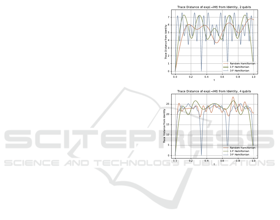
this way is given in Figure 1.

Figure 1: Plot of the trace distance between U (t) and I,

where U is generated respectively by a random hamiltonian

(in orange), a hamiltonian with period 1 (in green), and a

hamiltonian with period 3 (in blue), for 2 (up) and 4 (down)

qubits. Periodic hamiltonians are generated starting from

integer eigenvalues uniformly sampled in {−15,... ,15}.

3.3.1 Optimization and Practical Considerations

While the eigenvalues and unitary M can theoreti-

cally be optimized, this process requires efﬁcient gra-

dient computation and typically a supervised setting.

Such optimization may be impractical for anomaly

detection tasks, which are often unsupervised or semi-

supervised. Moreover, prior work (Baker et al., 2024)

has shown that random parameter selection in similar

kernels often performs comparably to optimized pa-

rameters, suggesting that optimization might not jus-

tify the additional complexity.

Randomly selected weights are commonly used

in other QML approaches, such as Quanvolutional

Neural Networks (Henderson et al., 2019). Addition-

ally, as discussed in (Mattern et al., 2021), evaluations

with trained and random parameters yield similar re-

Periodic Unitary Encoding for Quantum Anomaly Detection of Temporal Series

sults, indicating that parameter optimization may not

always provide signiﬁcant beneﬁts for QML models.

3.4 Resulting Kernel K

The ﬁnal step involves selecting the coefﬁcients of the

kernel K. This step determines how the instantaneous

kernels are combined to form the ﬁnal kernel deﬁned

in Equation 5. Two approaches can be employed to

select the coefﬁcients α

: heuristic selection and opti-

mization using Multiple Kernel Learning (MKL).

3.4.1 Heuristic Selection

The simplest approach involves selecting the coefﬁ-

cients randomly or based on predeﬁned properties.

For instance, using uniform weights α

= 1/L yields

an average kernel, which has been shown to perform

well in many contexts (Xu et al., 2013).

To incorporate periodicity, weights can be chosen

such that α

= α

i+P

, where P represents the period-

icity of the series. This ensures that values sampled

at intervals of P are evaluated equivalently. Formally,

for a translation of P steps, denoted as δ

, the kernel

satisﬁes:

K(x,y) = K(δ

(x),δ

(y)). (11)

This invariance under translations is particularly use-

ful for tasks where the starting time step of the se-

ries is irrelevant. For example, in a time series with

weekly periodicity, the series may start on different

days of the week without affecting the analysis.

3.4.2 Optimization via Multiple Kernel

Learning

The second approach involves using MKL tech-

niques to optimize the coefﬁcients α

based on a tar-

get property or function. A prominent example is

the EasyMKL algorithm (Aiolli and Donini, 2015),

which maximizes a speciﬁed metric between data

points. Speciﬁcally, it maximizes the distance be-

tween positive and negative examples with a unitary

norm vector holding the coefﬁcients of the Kernel’s

combination.

A key advantage of this approach is that the opti-

mization process is entirely classical, requiring no ac-

cess to quantum resources once the kernels are com-

puted. As a result, the proposed kernel remains within

the CSIM

class. However, it is important to note

that MKL techniques typically rely on supervised set-

tings, which may not be suitable for many anomaly

detection tasks.

4 EXPERIMENTAL DESIGN

To evaluate our proposed model, we addressed an

anomaly detection task for a time series with a given

periodicity. In particular, we considered the well-

known Taxi Request dataset

. This dataset contains

the number of taxi requests recorded by the NYC and

Limousine Commission from July 2014 to January

2015, and provides the aggregated count of passenger

at each 30 minutes interval. It presents 5 ”documented

anomalies”, corresponding to signiﬁcant events dur-

ing the tested period: the NYC Marathon (November

2, 2014), Thanksgiving (November 27, 2014), Christ-

mas (December 25, 2014), New Year’s Day (January

1, 2015), and a severe New England blizzard (January

27, 2015). For this reason, it provides a good ground

truth for evaluating anomaly detection algorithms.

We preprocessed the dataset with the following

steps:

• First, we divided the series in windows of size cor-

responding to 7 days;

• For each window, we label it as “anomalous” if it

contains one of the ﬁve anomalous days.

4.1 Tested Models

We compare our proposed model with periodic uni-

tary encoding with other One-Class SVMs using sev-

eral classical kernels, As a ﬁrst classical baseline, we

compare our model with periodic unitary encoding to

One-Class SVMs using several classical kernels that

do not take into account temporal properties. In par-

ticular, we evaluated classical SVMs built on linear,

polynomial, and Radial Basis Function kernels.

In addition, we evaluate a One-Class SVM model

based on the Dynamic Time Warping (DTW) (Berndt

and Clifford, 1994), a widely used distance for se-

quential pattern matching. The model implemented

uses as the kernel matrix the similarity values ob-

tained by inverting the distances, similarly to what

is done in (Shimodaira et al., 2001; Bahlmann et al.,

2002). However, is important to note that DTW is

not a Positive Deﬁnite Symmetric function, and thus

does not induce a proper kernel function (Lei and Sun,

2007).

As quantum models, we considered

• Quantum temporal kernel with Random Hamilto-

nian;

• Quantum temporal kernel with periodical unitary

of period 1 (1-P hamiltonian);

Accessible at https://www.kaggle.com/datasets/julien

jta/nyc-taxi-trafﬁc.

IQSOFT 2025 - 1st International Conference on Quantum Software

• Quantum temporal kernel with periodical unitary

of period 7 (7-P hamiltonian), corresponding to a

period equal to one day.

The Random Hamiltonian model is used as baseline

to evaluate the 7-P model. The 1-P model is used to

determine if variations in the performances depend on

the periodicity component, or just on the differences

in the generation of the kernel.

4.2 Implementation Details

Each model is trained only on non-anomalous data

(corresponding to weeks with no anomalous days).

After the training, the remaining data is split in a

small validation set, used to select hypeparameters,

and on test set, used for the ﬁnal evaluation. In details,

for each experiment, we ﬁrst split the non-anomalous

data with a 0.7, 0.3 ratio to obtain the train set. Vali-

dation and test sets are obtained with a split of 0.3,0.7

on the remaining samples, and contains both anoma-

lous and non-anomalous samples. Hyperparameters

selection (corresponding to the ν value and the thresh-

old value of the SVM) is performed by maximizing

the balanced accuracy of the model on the validation

set. This step does not require to recompute the ker-

nels, and can be done efﬁciently without using quan-

tum resources.

Quantum kernels are obtained with 2-qubits cir-

cuits, simulated in a noiseless environment with the

Qiskit library (Javadi-Abhari et al., 2024). Periodic

Hamiltonians are constructed starting from random

eigenvalues uniformly sampled in {−15, .. .,15}. The

data encoding, corresponding to U(x

) in the Equation

8, is the angle encoding R

(xπ). Each experiment is

repeated 30 times.

5 RESULTS

5.1 Performance Metrics

We evaluate the models using well-known metrics

such as Precision, Recall, F1-Score, and Balanced

Accuracy. Average results with standard deviation are

given in Table 1, and plotted in Figure 2.

5.1.1 Quantum Models

Among the quantum models, the 7-period Hamilto-

nian demonstrates the best performance, achieving

a balanced accuracy of 81.56% and an F1-Score of

73.33%. This indicates its superior ability to differen-

tiate between normal and anomalous data. In com-

parison, the 1-period Hamiltonian and the random

Hamiltonian models exhibit similar performances,

with balanced accuracies of 75.6% and 76.1%, re-

spectively, and slightly lower F1-Scores around 61%

and 63%. The 7-period Hamiltonian obtained also the

highest Precision and Recall compared to other quan-

tum models.

5.1.2 Classical Models

Classical methods such as the linear kernel, poly-

nomial kernel, and radial basis function (RBF) ker-

nel treat time series as simple vectors with L ele-

ments, disregarding temporal dependencies. Among

these, the RBF kernel achieves the highest precision

(94.1%) and balanced accuracy (86.9%), indicating

its ability to make reliable predictions with fewer false

positives. The polynomial kernel follows with a bal-

anced accuracy of 73% and an F1-Score of 60.4%,

showing moderate performance. The linear kernel

achieves a balanced accuracy of 71.6%, which is

lower than the RBF but still competitive.

On the other hand, Dynamic Time Warping, a

method speciﬁcally designed to account for temporal

dynamics, achieves a balanced accuracy of 85% and

an F1-Score of 80.2%. Despite obtaining the highest

Recall between tested models (equal to 80%), other

metrics are lower then RBF.

5.2 Discussion

The results demonstrate the importance of incorporat-

ing temporal information into model design. In par-

ticular, the 7-period Hamiltonian model consistently

outperformed both the random Hamiltonian, and the

1-period models, highlighting the value of leveraging

periodic structures in time series data. Is it interesting

to note that, even if the generation of the hamiltonian

between the Random Hamiltonian and the 1-P model

is different, they perform in a similar manner, show-

ing that the increased performance on the 7-P model

depends on selecting the correct period.

The 7-P model obtains Precision and Balanced

Accuracy competitive to the ones obtained by the

DTW model, which is, in general, expensive to com-

pute (Wang et al., 2010). However, RBF has a bet-

ter overall performance, suggesting that this particular

task do not require necessarily temporal understand-

ing.

6 CONCLUSION

In this work, we tackled the problem of anomaly de-

tection for temporal series with some form of season-

Periodic Unitary Encoding for Quantum Anomaly Detection of Temporal Series

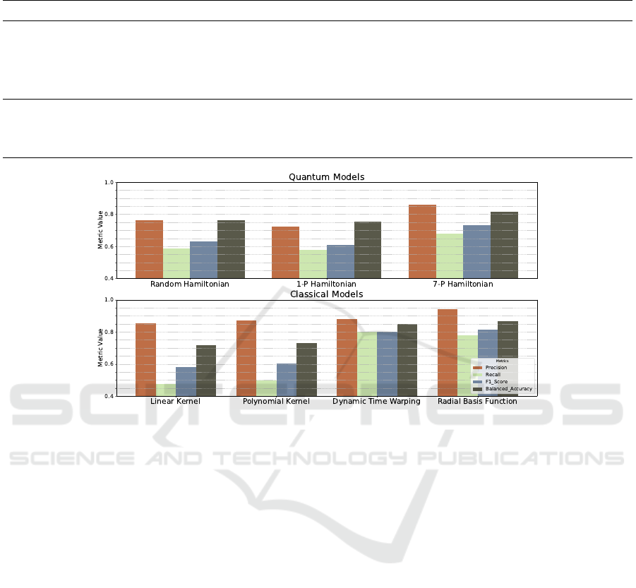
Table 1: Performance metrics of classical and quantum models on anomaly detection tasks. The table reports mean values

and standard deviations for Precision, Recall, F1 Score, and Balanced Accuracy.

Model Precision Recall F1 Score Balanced Accuracy

Linear Kernel 0.855 ± 0.275 0.478 ± 0.243 0.581 ± 0.218 0.716 ± 0.110

Polynomial Kernel 0.871 ± 0.268 0.500 ± 0.244 0.604 ± 0.222 0.730 ± 0.109

Dynamic Time Warping 0.882 ± 0.156 0.800 ± 0.241 0.802 ± 0.155 0.850 ± 0.111

Radial Basis Function 0.941 ± 0.122 0.778 ± 0.295 0.814 ± 0.222 0.869 ± 0.153

Random Hamiltonian 0.764 ± 0.376 0.589 ± 0.358 0.630 ± 0.329 0.761 ± 0.170

1-P Hamiltonian 0.721 ± 0.396 0.578 ± 0.381 0.610 ± 0.356 0.756 ± 0.185

7-P Hamiltonian 0.860 ± 0.272 0.678 ± 0.297 0.733 ± 0.263 0.816 ± 0.148

Figure 2: Barplot of average Precision, Recall, F1-Score, and Balanced Accuracy of the considered models.

ality. We proposed a Periodic Unitary Encoding for

a quantum kernel model that leverages the seasonal-

ity of temporal series to provide a better classical data

representation. This unitary transformation is induced

by a Hamiltonian constructed from a set of coprime

eigenvalues.

Testing our method against an anomaly detection

task showed that, by leveraging the correct period of

the data, the quantum model obtained better results.

Nevertheless, a comparison of our results with those

obtained using RBF indicates that the latter achieves

superior performance. Given that RBF does not uti-

lize temporal correlation, we can suppose that the

task we addressed is not strongly dependent on time-

related information. Therefore it would be worth in-

vestigating if our approach outperforms other quan-

tum models also when addressing tasks that have a

deeper connection to time-related properties.

To conclude, it is interesting to note that the pro-

posed periodic unitary encoding has potential appli-

cations beyond anomaly detection, offering a ﬂexible

approach for tasks where the quantum representation

of classical data must satisfy speciﬁc properties, such

as equivariance under translations (Bronstein et al.,

2017).

By introducing this method, we provide a step

forward in exploring how domain-speciﬁc knowledge

can inform quantum data encoding, contributing to

the advancement of Quantum Machine Learning in

practical and meaningful ways.

REFERENCES

Aiolli, F. and Donini, M. (2015). Easymkl: a scalable

multiple kernel learning algorithm. Neurocomputing,

169:215–224. Learning for Visual Semantic Under-

standing in Big Data ESANN 2014 Industrial Data

Processing and Analysis.

Alam, S., Sonbhadra, S. K., Agarwal, S., and Nagabhushan,

P. (2020). One-class support vector classiﬁers: A sur-

vey. Knowledge-Based Systems, 196:105754.

Amer, M., Goldstein, M., and Abdennadher, S. (2013). En-

hancing one-class support vector machines for unsu-

pervised anomaly detection. pages 8–15.

Bahlmann, C., Haasdonk, B., and Burkhardt, H. (2002).

Online handwriting recognition with support vector

machines - a kernel approach. In Proceedings Eighth

International Workshop on Frontiers in Handwriting

Recognition, pages 49–54.

Baker, J., Park, G., Yu, K., Ghukasyan, A., Goktas, O., and

IQSOFT 2025 - 1st International Conference on Quantum Software

Kumar, S. (2024). Parallel hybrid quantum-classical

machine learning for kernelized time-series classiﬁca-

tion. Quantum Machine Intelligence, 6.

Belis, V., Wo

zniak, K., Puljak, E., Barkoutsos, P., Disser-

tori, G., Grossi, M., Pierini, M., Reiter, F., Tavernelli,

I., and Vallecorsa, S. (2024). Quantum anomaly de-

tection in the latent space of proton collision events at

the lhc. Communications Physics, 7.

Benitez, J. and Thome, N. (2006). k -group periodic ma-

trices. SIAM Journal on Matrix Analysis and Applica-

tions, 28:9–25.

Berndt, D. and Clifford, J. (1994). Using dynamic time

warping to ﬁnd patterns in time series. In KDD work-

shop, volume 10, pages 359–370.

Bronstein, M., Bruna, J., LeCun, Y., Szlam, A., and Van-

dergheynst, P. (2017). Geometric deep learning: go-

ing beyond euclidean data. IEEE Signal Processing

Magazine, 34(4):18–42.

Buhrman, H., Cleve, R., Watrous, J., and de Wolf, R.

(2001). Quantum ﬁngerprinting. Phys. Rev. Lett.,

87:167902.

Cerezo, M., Arrasmith, A., Babbush, R., Benjamin, S.,

Endo, S., Fujii, K., McClean, J., Mitarai, K., Yuan, X.,

Cincio, L., and Coles, P. (2021a). Variational quantum

algorithms. Nature Reviews Physics, 3(9):625–644.

Cerezo, M., Larocca, M., Garc

ıa-Mart

ın, D., Diaz, N.,

Braccia, P., Fontana, E., Rudolph, M., Bermejo, P.,

Ijaz, A., Thanasilp, S., Anschuetz, E., and Holmes, Z.

(2024). Does provable absence of barren plateaus im-

ply classical simulability? or, why we need to rethink

variational quantum computing.

Cerezo, M., Sone, A., Volkoff, T., Cincio, L., and Coles, P.

(2021b). Cost function dependent barren plateaus in

shallow parametrized quantum circuits. Nature Com-

munications, 12.

Crooks, G. (2019). Gradients of parameterized quantum

gates using the parameter-shift rule and gate decom-

position.

Darban, Z., Webb, G., Pan, S., Aggarwal, C., and Salehi,

M. (2024). Deep learning for time series anomaly de-

tection: A survey. ACM Comput. Surv., 57(1).

onen, M. and Alpaydin, E. (2011). Multiple kernel learn-

ing algorithms. Journal of Machine Learning Re-

search, 12(64):2211–2268.

Havl

cek, V., C

orcoles, A., Temme, K., Harrow, A., Kan-

dala, A., Chow, J., and Gambetta, J. (2019). Super-

vised learning with quantum-enhanced feature spaces.

Nature, 567(7747):209–212.

Henderson, M., Shakya, S., Pradhan, S., and Cook, T.

(2019). Quanvolutional neural networks: Powering

image recognition with quantum circuits.

Holmes, Z., Sharma, K., Cerezo, M., and Coles, P. (2022).

Connecting ansatz expressibility to gradient magni-

tudes and barren plateaus. PRX Quantum, 3:010313.

Incudini, M., Lizzio Bosco, D., Martini, F., Grossi, M.,

Serra, G., and Di Pierro, A. (2024). Automatic and

effective discovery of quantum kernels. IEEE Trans-

actions on Emerging Topics in Computational Intelli-

gence, PP:1–10.

Javadi-Abhari, A., Treinish, M., Krsulich, K., Wood, C.,

Lishman, J., Gacon, J., Martiel, S., Nation, P., Bishop,

L., Cross, A., Johnson, B., and Gambetta, J. (2024).

Quantum computing with Qiskit.

Jeswal, S. and Chakraverty, S. (2018). Recent develop-

ments and applications in quantum neural network: A

review. Archives of Computational Methods in Engi-

neering, 26:793 – 807.

Kim, Y., Eddins, A., Anand, S., Wei, K., Berg, E., Rosen-

blatt, S., Nayfeh, H., Wu, Y., Zaletel, M., Temme, K.,

and Kandala, A. (2023). Evidence for the utility of

quantum computing before fault tolerance. Nature,

618:500–505.

Lei, H. and Sun, B. (2007). A study on the dynamic time

warping in kernel machines. In 2007 Third Interna-

tional IEEE Conference on Signal-Image Technolo-

gies and Internet-Based System, pages 839–845.

Liu, Y., Arunachalam, S., and Temme, K. (2021). A rig-

orous and robust quantum speed-up in supervised ma-

chine learning. Nature Physics, 17:1–5.

Mattern, D., Martyniuk, D., Willems, H., Bergmann, F., and

Paschke, A. (2021). Variational Quanvolutional Neu-

ral Networks with enhanced image encoding.

Minh, H. Q., Niyogi, P., and Yao, Y. (2006). Mercer’s theo-

rem, feature maps, and smoothing. In Lugosi, G. and

Simon, H. U., editors, Learning Theory, pages 154–

168, Berlin, Heidelberg. Springer Berlin Heidelberg.

Mishra, N., Kapil, M., Rakesh, H., Anand, A., Mishra,

N., Warke, A., Sarkar, S., Dutta, S., Gupta, S.,

Prasad Dash, A., Gharat, R., Chatterjee, Y., Roy,

S., Raj, S., Kumar Jain, V., Bagaria, S., Chaud-

hary, S., Singh, V., Maji, R., Dalei, P., Behera,

B. K., Mukhopadhyay, S., and Panigrahi, P. K. (2021).

Quantum machine learning: A review and current sta-

tus. In Sharma, N., Chakrabarti, A., Balas, V. E., and

Martinovic, J., editors, Data Management, Analytics

and Innovation, pages 101–145. Springer Singapore.

Nielsen, M. A. and Chuang, I. L. (2010). Quantum Com-

putation and Quantum Information: 10th Anniversary

Edition. Cambridge University Press.

Peral-Garc

ıa, D., Cruz-Benito, J., and Garc

ıa-Pe

nalvo, F.

(2024). Systematic literature review: Quantum ma-

chine learning and its applications. Computer Science

Review, 51:100619.

Ragone, M., Braccia, P., Nguyen, Q., Schatzki, L., Coles,

P., Sauvage, F., Larocca, M., and Cerezo, M. (2023).

Representation theory for geometric quantum ma-

chine learning.

Rath, M. and Date, H. (2024). Quantum data encoding:

a comparative analysis of classical-to-quantum map-

ping techniques and their impact on machine learning

accuracy. EPJ Quantum Technology, 11.

Rebentrost, P., Mohseni, M., and Lloyd, S. (2014). Quan-

tum support vector machine for big data classiﬁcation.

Physical Review Letters, 113(13).

Ruder, S. (2017). An overview of gradient descent opti-

mization algorithms.

Schnabel, J. and Roth, M. (2024). Quantum kernel methods

under scrutiny: A benchmarking study.

Periodic Unitary Encoding for Quantum Anomaly Detection of Temporal Series

Schuld, M. and Killoran, N. (2019). Quantum machine

learning in feature hilbert spaces. Physical Review

Letters, 122(4).

Shawe-Taylor, J. and Sun, S. (2014). Kernel Methods and

Support Vector Machines, volume 1, pages 857–881.

Shimodaira, H., Noma, K., Nakai, M., and Sagayama, S.

(2001). Dynamic time-alignment kernel in support

vector machine. In Dietterich, T., Becker, S., and

Ghahramani, Z., editors, Advances in Neural Informa-

tion Processing Systems, volume 14. MIT Press.

Uvarov, A. and Biamonte, J. (2021). On barren plateaus

and cost function locality in variational quantum al-

gorithms. Journal of Physics A: Mathematical and

Theoretical, 54(24):245301.

Wang, S., Fontana, E., Cerezo, M., Sharma, K., Sone, A.,

Cincio, L., and Coles, P. (2021). Noise-induced barren

plateaus in variational quantum algorithms. Nature

Communications, 12.

Wang, X., Ding, H., Trajcevski, G., Scheuermann, P., and

Keogh, E. (2010). Experimental comparison of rep-

resentation methods and distance measures for time

series data.

Wang, Y. and Liu, J. (2024). A comprehensive review of

quantum machine learning: from nisq to fault toler-

ance. Reports on Progress in Physics, 87(11).

Wierichs, D., Izaac, J., Wang, C., and Lin, C. (2022).

General parameter-shift rules for quantum gradients.

Quantum, 6.

Xu, X., Tsang, I., and Xu, D. (2013). Soft margin multiple

kernel learning. 24(5):749 – 761.

Yousif, M., Mohammed, M., Celik, M., Hamdoon, A., Jas-

sim, R., and Abdullah, N. (2024). Periodicity analysis

of most time series methods: A review. In 2024 8th

International Symposium on Multidisciplinary Studies

and Innovative Technologies (ISMSIT), pages 1–7.

IQSOFT 2025 - 1st International Conference on Quantum Software