Trajectory Planning for a Knuckle Boom Crane Using Differential

Dynamic Programming

Chair of Materials Handling, Material Flow, Logistics, Technical University of Munich, Boltzmannstraße 15, 85748

Garching bei M

unchen, Germany

Keywords:

Knuckle Boom Crane, Trajectory Planning, Differential Dynamic Programming, Kinematic Constraints.

Abstract:

Knuckle boom cranes are widely used in numerous applications, making effective obstacle avoidance trajec-

tory planning critical for automation. However, the cranes’ inherent kinematic constraints pose signiﬁcant

challenges to designing and optimizing such trajectory planning problems. In this study, we develop a tra-

jectory planning method that addresses obstacle avoidance under these kinematic constraints by employing

Differential Dynamic Programming (DDP). We ﬁrst derive an explicit Euler-based dynamic model of the

crane, integrating Baumgarte stabilization to suppress kinematic constraint violations within the DDP frame-

work. Additionally, a relaxed log-barrier function is introduced to handle both states and obstacle-avoidance

constraints during trajectory planning. Comparative numerical simulations with the Ipopt solver demonstrate

the effectiveness of the proposed approach in achieving obstacle avoidance and constraints suppression.

1 INTRODUCTION

The knuckle boom crane is a representative type of

engineering equipment with a wide range of appli-

cations, including logistics, construction, and indus-

trial manufacturing. Among the areas, knuckle boom

cranes are required to efﬁciently transport heavy pay-

loads in complex working environments. However,

as a typical underactuated mechanical system, rapid

crane movements involving large acceleration or de-

celeration often lead to undesirable payload oscilla-

tions, posing signiﬁcant challenges for manual crane

operation. To address this issue, the development

of efﬁcient and safe trajectory planning methods for

knuckle boom cranes has attracted growing attentions

from both industry and academia.

In recent years, numerous studies have made sig-

niﬁcant progress in crane trajectory planning. For the

typical underactuated overhead crane system, (Zhang

et al., 2021) employed the principle of differential

ﬂatness to generate a time-optimal trajectory for a

planner double-pendulum overhead crane, thereby

improving the transportation efﬁciency. In (Thi et al.,

2024), the differential ﬂatness-based trajectory plan-

ning method was extended to a three-dimensional

overhead crane. Furthermore, (Li et al., 2022) an-

alyzed minimum-time, minimum-energy, and com-

bined optimal time-energy trajectory planning for an

overhead crane with pendulum-sloshing dynamics by

formulating the problem under a quasi-convex op-

timization framework. Another typical crane sys-

tem was investigated in (Farrage et al., 2023), which

proposed a three-dimensional rotary crane trajectory

planning method using the A* algorithm to gener-

ate an obstacle-avoidance path, followed by a time-

optimal trajectory solution under crane dynamics and

load-sway constraints. Besides, a neural network-

based time-optimal trajectory planning method for

rotary cranes was further developed in (Zhu et al.,

2023). However, compared to overhead or rotary

cranes, knuckle boom cranes typically feature a more

complex mechanical structure with higher dimension-

ality and greater ﬂexibility, which complicates the

process of trajectory planning.

As an efﬁcient indirect trajectory planning method

characterized by its rapid convergence and relatively

low computational cost, Differential Dynamic Pro-

gramming (DDP) has been utilized in many ﬁelds,

including quadruped robots (Li and Wensing, 2020;

Kim et al., 2022; Mastalli et al., 2020), autonomous

driving (Chen et al., 2019; Huang et al., 2023; Lee

et al., 2022), and robotic manipulators (Zimmermann

et al., 2021; Wang et al., 2023). The theoretical

foundation of DDP, as presented in (Zheng et al.,

2021), is based on the Bellman optimality principle

and second-order Taylor expansions, effectively split

Zhiwei Wang, Lingchong Gao, Michael Kleeberger and Johannes Fottner

Wang, Z., Gao, L., Kleeberger, M., Fottner and J.

Trajectory Planning for a Knuckle Boom Crane Using Differential Dynamic Programming.

DOI: 10.5220/0013522000003970

In Proceedings of the 15th International Conference on Simulation and Modeling Methodologies, Technologies and Applications (SIMULTECH 2025), pages 62-69

ISBN: 978-989-758-759-7; ISSN: 2184-2841

2 CRANE DYNAMICS

Referring to (Martin and Irani, 2021), a simpliﬁed

knuckle boom crane is illustrated in Fig. 1, in this

model, the crane system is modelled as a rigid multi-

body system, where the distributed mass payload is

attached to the tip of the crane boom via a rigid, mass-

less cable.

To describe the motion of the crane system, a set

of generalized coordinates is deﬁned:

𝑞

𝑞 =

(

𝜃

, 𝜃

, 𝑑

, 𝜃

, 𝑑

, 𝜃

, 𝑑

, 𝜙

)

⊤

, (1)

where 𝜃

denotes the rotation angle of the column, 𝜃

denotes the relative rotation of the inner boom with re-

spect to the column. Correspondingly, the inner boom

hydraulic actuator consists of a cylinder rotates an an-

gle 𝜃

and a rob translates a distance 𝑑

. Similar with

the inner boom, the relative rotation of the outer boom

is represented by 𝜃

, the rotation and the translation of

the outer boom hydraulic actuator are represented by

𝜃

and 𝑑

, respectively. In addition, the translation of

the extension boom is expressed by 𝑑

, while 𝜙

and

𝜙

are utilized to describe the oscillation angles of the

payload.

Without loss of generality, the dynamic equations

that govern the motion of the crane system can be

expressed as:

𝑀

(

𝑞

)

𝑞

𝑞 + 𝚽

⊤

𝑞

𝜆

𝜆 = 𝐹

𝐹

(

𝑞

𝑞,

𝑞

)

+ 𝐵

𝐵

𝐵𝑢

𝑢

𝑢, (2)

𝚽

(

𝑞

)

= 0

0, (3)

where 𝑀

𝑀

𝑀 ∈ R

10×10

denotes the generalized mass ma-

trix, 𝐹

𝐹

𝐹 ∈ R

represents the generalized force vector,

which includes Coriolis and gravity terms. The con-

trol vector is given by 𝑢

𝑢

𝑢 ∈ R

, while 𝐵

𝐵

𝐵 ∈ R

10×4

isthe

transformation matrix of the control vector, 𝚽 ∈ R

represents the kinematic constraints, 𝚽

𝑞

∈ R

10×4

the Jacobian matrix of the kinematic constraints, and

𝜆

𝜆 ∈ R

represents the corresponding Lagrange multi-

pliers.

3 CRANE TRAJECTORY

PLANNING

In this section, the dynamic equations of the con-

strained crane system described in Section 2 are trans-

formed into an explicit Euler dynamic model, fa-

cilitating its incorporation into the DDP framework.

Then, the optimal trajectory planning problem for the

knuckle boom crane is formulated.

3.1 Kinematic Constraints Elimination

To address the kinematic constraints in the knuckle

boom crane system, the constraints at the velocity and

the trajectory planning task into smaller subproblems

at each time step. However, despite its high effec-

tiveness for unconstrained problems, DDP encounters

difﬁculties in handling constraints. In (Kazdadi et al.,

2021), an augmented Lagrangian method was intro-

duced to handle equality-constrained DDP trajectory

planning. In (Jallet et al., 2022), a more generic

primal-dual augmented Lagrangian strategy for deal-

ing with equality and inequality constraints in non-

linear DDP problems was proposed, while (Aoyama

et al., 2021) investigated penalty methods and active-

set methods to tackle constrained DDP trajectory

planning problems.

In contrast to the dynamic system featuring ex-

ternal constraints, knuckle boom cranes feature a set

of inherent kinematic equality constraints originating

from their mechanical structure, commonly known as

closed-loop constraints. It is often necessary to intro-

duce constraint forces or include Lagrange multipli-

ers in the construction of dynamic equations, form-

ing differential-algebraic equations (DAEs), to ensure

that the closed-loop kinematic relations are satisﬁed.

This complicates the design and reduces the optimiza-

tion efﬁciency of DDP-based trajectory planning for

knuckle boom cranes.

Motivated by the aforementioned analysis, the

main contributions of this paper are as follows:

• The standard Lagrange multiplier method is com-

bined with Baumgarte stabilization to embed con-

straint equations into the crane system dynamics,

thereby converting DAEs into a more convenient

ODE form for DDP algorithm design.

• Additionally, a relaxed log-barrier function-based

DDP algorithm is employed to handle state con-

straints and obstacle avoidance constraints during

knuckle boom crane trajectory planning.

• The effectiveness and constraint violation sup-

pression of the proposed method are demonstrated

through several numerical simulations.

The paper is organized as follows. In Section 2,

the dynamic equations for the knuckle boom crane

are presented. In Section 3, the standard Lagrange

method is combined with Baumgarte stabilization to

transform the crane dynamics with kinematic con-

straints into a general ODE form. Additionally, a re-

laxed log-barrier function is introduced to handle state

constraints and obstacle avoidance during trajectory

planning. The effectiveness of the proposed method

is validated through numerical cases in Section 4. Fi-

nally, Section 5 presents conclusions and outlines po-

tential directions for future research.

Trajectory Planning for a Knuckle Boom Crane Using Differential Dynamic Programming

𝒙

𝒚

𝒛

𝜃

𝑑

𝜃

𝑑

𝜃

𝑑

𝜙

𝒙

𝒚

𝒛

𝑜

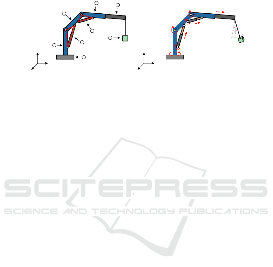
Figure 1: Knuckle boom crane: (a) Crane components: 1. Column; 2. Inner boom; 3. Outer boom; 4. Extension boom; 5.

Base; 6. Inner boom hydraulic actuator; 7. Outer boom hydraulic actuator; 8. Payload; (b) Kinematics depiction.

acceleration levels in the crane system derived from

Eq. (3) can be further expressed as:

𝚽

𝑞

𝑞 = 0

0, (4)

𝚽

𝑞

𝑞 +

𝚽

𝑞

𝑞 = 0

0. (5)

The acceleration constraints formulated in Eq. (5)

introduce auxiliary equations equal in number to the

Lagrange multipliers.

By integrating these constraints with the system

dynamic equations Eq. (2) with the Baumgarte sta-

bilization method, the constrained dynamic system is

reformulated as:



𝑀

𝑀 𝚽

⊤

𝑞

𝚽

𝑞



𝑞

𝜆





𝐹

𝐹 + 𝐵

𝐵

𝐵𝑢

𝑢

−

𝚽

𝑞

𝑞 − 2𝜉

𝚽 −

−

− 𝜉

𝚽



, (6)

where 𝜉

is the damping coeﬃcient and 𝜉

is a positive

stiﬀness coeﬃcient.

Eliminating the acceleration vector

𝑞

𝑞 in Eq. (6),

the Lagrange multiplier 𝜆

𝜆

𝜆 can be explicitly expressed

as:

𝜆

𝜆 =



𝚽

𝑞

𝑀

−1

𝚽

⊤

𝑞



−1

𝚽

𝑞

𝑀

−1

(

𝐹

𝐹 + 𝐵

𝐵

𝐵𝑢

𝑢

)



𝚽

𝑞

𝑀

−1

𝚽

⊤

𝑞



−1



𝚽

𝑞

𝑞 + 2𝜉

𝚽 + 𝜉

𝚽



(7)

Substituting Eq. (7) into Eq. (6) yields the con-

strained system acceleration:

𝑞

𝑞 =

𝑀

−1

− 𝑀

𝑀

−1

𝚽

⊤

𝑞



𝚽

𝑞

𝑀

−1

𝚽

⊤

𝑞



−1

𝚽

𝑞

𝑀

−1

(

𝐹

𝐹 + 𝐵

𝐵

𝐵𝑢

𝑢

)

− 𝑀

𝑀

−1

𝚽

⊤

𝑞



𝚽

𝑞

𝑀

−1

𝚽

⊤

𝑞



−1



𝚽

𝑞

𝑞 + 2𝜉

𝚽 + 𝜉

𝚽



(8)

Note that this transformation for solving the dy-

namic equations is often referred to as the standard

Lagrange multipliers method (Marques et al., 2017).

Over a small time interval Δ𝑡 = 𝑡

𝑘+1

− 𝑡

𝑘

, the sys-

tem dynamics are discretized using the Explicit Euler

method, resulting in:

𝑥

𝑘+1

= 𝑓

𝑓

(

𝑥

𝑘

, 𝑢

𝑢

𝑘

)

= 𝑥

𝑥

𝑘

𝑥

𝑘

Δ𝑡, (9)

where 𝑘 is the time step, 𝑥

𝑥

⊤

𝑘

[

𝑞

⊤

(𝑡

𝑘

𝑞

⊤

(𝑡

𝑘

)

]



𝑞

⊤

𝑘

𝑞

⊤

𝑘



denotes the state vector, and the control in-

puts 𝑢

𝑢

𝑘

is assumed to remain constant throughout each

interval.

3.2 Optimization Problem Formulation

Trajectory planning for the knuckle boom crane aims

to determine an optimal trajectory for payload trans-

portation, ensuring safety, smoothness, and precision.

Consequently, the optimization problem is formulated

as follows:

min

𝑢

0:𝑁 −1

(

𝑥

𝑁

− 𝑥

𝑥

)

⊤

𝑄

(

𝑥

𝑁

− 𝑥

𝑥

)

𝑛−1



𝑘=0



(

𝑥

𝑘

− 𝑥

𝑥

)

⊤

𝑄

(

𝑥

𝑘

− 𝑥

𝑥

)

+ 𝑢

𝑢

⊤

𝑘

𝑅

𝑅𝑢

𝑢

𝑘



(10)

where 𝑄

𝑄

𝑄 ∈ R

20×20

, 𝑅

𝑅

𝑅 ∈ R

20×20

and 𝑄

𝑄

∈ R

20×20

are

weighting matrices, with 𝑄

𝑄

𝑄 and 𝑄

𝑄

being positive

semi-deﬁnite and 𝑅

𝑅

𝑅 being positive deﬁnite. 𝑥

𝑥

∈ R

represents the target state of the crane.

The knuckle boom crane is typically subject to

several inequality constraints imposed by mechanical

and actuator limitations, including hydraulic cylinder

extensions, forces, and payload oscillations, which can

be expressed as:

𝑥

min

≤ 𝑥

𝑥

𝑘

≤ 𝑥

𝑥

max

, (11)

𝑢

min

≤ 𝑢

𝑢

𝑘

≤ 𝑢

𝑢

max

, (12)

where 𝑥

𝑥

min

and 𝑥

𝑥

max

represent the lower and upper

bounds of the states, respectively, while 𝑢

𝑢

min

and 𝑢

𝑢

max

denote the lower and upper bounds of the control in-

puts, respectively.

Furthermore, the payload must be constrained

within a predeﬁned safe region to ensure collision

avoidance with obstacles, thereby guaranteeing the

safety and feasibility of the planned trajectory, this

can be formulated as:

𝑑



𝑥

𝑘

, 𝑝

𝑝

𝛾



≥ 𝑑

safe

, 𝛾 = 0, . . . , 𝐵, (13)

SIMULTECH 2025 - 15th International Conference on Simulation and Modeling Methodologies, Technologies and Applications

where 𝑑



𝑥

𝑘

, 𝑝

𝑝

𝛾



represents the Euclidean distance

between the payload and the surface of the 𝛾

obsta-

cle, 𝑝

𝑝

𝛾

denotes the position of the 𝛾

obstacle, 𝑑

safe

represents the predeﬁned safety margin, and 𝐵 is the

total number of obstacles.

Considering the crane dynamics described in Eq.

(9), the cost function in Eq. (10), and inequality con-

straints described from Eq. (11) to Eq. (13), the

trajectory planning of the crane can be formulated in

an optimization problem as follows:

min

𝑈

𝐽

(

𝑋

𝑋,𝑈

𝑈

)

= min

𝑈



𝑙

𝑁

(

𝑥

𝑁

)

𝑁 −1

𝑘=0

𝑙

𝑘

(

𝑥

𝑘

, 𝑢

𝑢

𝑘

)



(14a)

𝑥

𝑘+1

= 𝑓

𝑓

(

𝑥

𝑘

, 𝑢

𝑢

𝑘

)

, 𝑘 = 0, . . . , 𝑁 − 1, (14b)

𝑔

𝑘

(

𝑥

𝑘

, 𝑢

𝑢

𝑘

)

> 0, (14c)

where 𝑙

𝑘

and 𝑙

𝑁

represent the stage and terminal cost

terms of Eq. (10),

{

𝑋

𝑋,𝑈

𝑈

}

is a sequence of sys-

tem states 𝑋

𝑋

𝑋 :=

{

𝑥

, 𝑥

𝑥

, . . . , 𝑥

𝑥

𝑁

}

and control inputs

𝑈

𝑈 :=

{

𝑢

, 𝑢

𝑢

, . . . , 𝑢

𝑢

𝑁 −1

}

, besides, 𝑔

𝑔

𝑘

(

𝑥

𝑘

, 𝑢

𝑢

𝑘

)

∈ R

𝑚

represents a general formulation of inequality con-

straints, incorporating both state constraints and ob-

stacle avoidance constraints.

3.3 Inequality-Constrained Diﬀerential

Dynamic Programming

For the inequality-constrained optimization problem

described in Eq. (14a), a well-established relaxed

log-barrier function method (Grandia et al., 2019) is

employed to transform the problem into an uncon-

strained optimization framework. Consequently, the

cost function in Eq. (10) is modiﬁed as:

min

𝑢

0:𝑁 −1

𝐽

(

𝑋

𝑋,𝑈

𝑈

)

= 𝑙

𝑁

(

𝑥

𝑁

, 𝑢

𝑢

𝑁

)

𝑁 −1



𝑘=0

𝑙

𝑘

(

𝑥

𝑘

, 𝑢

𝑢

𝑘

)

+ 𝑏

𝑘

(

𝑥

𝑘

, 𝑢

𝑢

𝑘

)

(15)

where barrier function 𝑏

𝑘

(

𝑥

𝑘

, 𝑢

𝑢

𝑘

)

is introduced:

𝑏

𝑘

(

𝑥

𝑘

, 𝑢

𝑢

𝑘

)











−𝜔

𝑚

𝑗=1



𝑔

𝑘, 𝑗

(

𝑥

𝑘

, 𝑢

𝑢

𝑘

)



, 𝑔

𝑔

𝑘

(

𝑥

𝑘

, 𝑢

𝑢

𝑘

)

≥ 𝛿,

𝑚

𝑗=1

𝛽



𝑔

𝑘, 𝑗

(

𝑥

𝑘

, 𝑢

𝑢

𝑘

)

, 𝛿



, 𝑔

𝑔

𝑘

(

𝑥

𝑘

, 𝑢

𝑢

𝑘

)

< 𝛿,

(16)

where 𝜔 > 0 and 𝛿 > 0 are penalty parameters, and

function 𝛽



𝑔

𝑘, 𝑗

(

𝑥

𝑘

, 𝑢

𝑢

𝑘

)

, 𝛿



is deﬁned as:

𝛽



𝑔

𝑘, 𝑗

(

𝑥

𝑘

, 𝑢

𝑢

𝑘

)

, 𝛿



𝜔





𝑔

𝑘, 𝑗

(

𝑥

𝑘

,𝑢

𝑢

𝑘

)

−2𝛿

𝛿



− 1



− 𝜔 ln(𝛿).

(17)

To evaluate the cost function in Eq. (15) cumula-

tively, the cost-to-go function is deﬁned:

𝐽

𝑘

(

𝑥

𝑘

, 𝑢

𝑢

𝑘

)

= 𝑙

𝑁

(

𝑥

𝑁

,𝜆

𝜆

𝑁

)

𝑁 −1



𝑗=𝑘+1

𝑙

𝑗



𝑥

𝑗

, 𝑢

𝑢

𝑗



. (18)

Thus, the value function, which represents the op-

timal cost-to-go, is given by:

𝑉

𝑘

(

𝑥

𝑘

)

= min

𝑢

𝑘

𝐽

𝑘

(

𝑥

𝑘

, 𝑢

𝑢

𝑘

)

. (19)

According to the Bellman optimality principle, the

recurrence relationship of the value function in back-

ward pass of DDP can be expressed as:

𝑉

𝑁

(

𝑥

𝑁

)

= 𝑙

𝑁

(

𝑥

𝑁

)

, (20)

𝑉

𝑘

(

𝑥

𝑘

)

= min

𝑢

𝑘

[

𝑙

𝑘

(

𝑥

𝑘

, 𝑢

𝑢

𝑘

)

+𝑉

𝑘+1

(

𝑥

𝑖+1

)]

. (21)

To evaluate the contribution of a speciﬁc control

action to the overall cost, the action-value function is

further employed:

𝑄

𝑘

(

𝑥

𝑘

, 𝑢

𝑢

𝑘

)

= 𝑙

𝑘

(

𝑥

𝑘

, 𝑢

𝑢

𝑘

)

+𝑉

𝑘+1

(

𝑥

𝑘+1

)

. (22)

Instead of solving the optimization problem glob-

ally, DDP performances a local second-order Taylor

series approximation of value function 𝑉

𝑘

, that is

𝛿𝑉

𝑘

≈ 𝑉

⊤

𝑥

𝑥,𝑘

𝛿𝑥

𝑥

𝑘

𝛿𝑥

𝑥

⊤

𝑘

𝑉

𝑥

𝑥𝑥

𝑥

𝑥,𝑘

𝛿𝑥

𝑥

𝑘

, (23)

where 𝑉

𝑥

𝑥𝑥

𝑥

𝑥,𝑘

and 𝑉

𝑥

𝑥,𝑘

are the Hessian and gradient

of the cost-to-go function at time step 𝑘, respectively.

Following Eq. (20), the second order expansion of the

value function at the terminal time are 𝑉

𝑥

𝑥, 𝑁

= 𝑙

𝑥

𝑥,

,𝑁

and 𝑉

𝑥

𝑥𝑥

𝑥

𝑥, 𝑁

= 𝑙

𝑥

𝑥𝑥

𝑥

𝑥,

,𝑁

Likewise, the second-order Taylor approximation

of the action-value function about the current nominal

trajectory is:

𝑄

𝑘



𝑥

𝑘

, 𝑢

𝑢

𝑘



≈ 𝑄

𝑘



𝑥

𝑘

, 𝑢

𝑢

𝑘



+ 𝑄

⊤

𝑥

𝑥,𝑘

𝛿𝑥

𝑥

𝑘

+ 𝑄

⊤

𝑢

𝑢, 𝑘

𝛿𝑢

𝑢

𝑘



𝛿𝑥

𝑥

𝑘

𝛿𝑢

𝑢

𝑘



⊤



𝑄

𝑥

𝑥𝑥

𝑥

𝑥,𝑘

𝑄

𝑥

𝑥𝑢

𝑢

𝑢, 𝑘

𝑄

𝑢

𝑢𝑥

𝑥

𝑥,𝑘

𝑄

𝑢

𝑢𝑢

𝑢

𝑢, 𝑘



𝛿𝑥

𝑥

𝑘

𝛿𝑢

𝑢

𝑘



(24)

where 𝑥

𝑥

𝑘

and 𝑢

𝑢

𝑘

represent the nominal state trajectory

and control trajectory, the partial derivatives terms of

𝑄

𝑘

are given by:

𝑄

𝑥

𝑥,𝑘

= 𝑙

𝑥

𝑥,𝑘

+ 𝑓

𝑓

⊤

𝑥

𝑥,𝑘

𝑉

𝑥

𝑥,𝑘+1

, (25)

𝑄

𝑢

𝑢, 𝑘

= 𝑙

𝑢

𝑢, 𝑘

+ 𝑓

𝑓

⊤

𝑢

𝑢, 𝑘

𝑉

𝑥

𝑥,𝑘+1

, (26)

𝑄

𝑥

𝑥𝑥

𝑥

𝑥,𝑘

= 𝑙

𝑥

𝑥𝑥

𝑥

𝑥,𝑘

+ 𝑓

𝑓

⊤

𝑥

𝑥,𝑘

𝑉

𝑥

𝑥𝑥

𝑥

𝑥,𝑘+1

𝑓

𝑥

𝑥,𝑘

+𝑉

𝑥

𝑥,𝑘+1

𝑓

𝑥

𝑥𝑥

𝑥

𝑥,𝑘

(27)

𝑄

𝑢

𝑢𝑢

𝑢

𝑢, 𝑘

= 𝑙

𝑢

𝑢𝑢

𝑢

𝑢, 𝑘

+ 𝑓

𝑓

⊤

𝑢

𝑢, 𝑘

𝑉

𝑥

𝑥𝑥

𝑥

𝑥,𝑘+1

𝑓

𝑢

𝑢, 𝑘

+𝑉

𝑥

𝑥,𝑘+1

𝑓

𝑢

𝑢𝑢

𝑢

𝑢, 𝑘

(28)

𝑄

𝑢

𝑢𝑥

𝑥

𝑥,𝑘

= 𝑙

𝑢

𝑢𝑥

𝑥

𝑥,𝑘

+ 𝑓

𝑓

⊤

𝑢

𝑢, 𝑘

𝑉

𝑥

𝑥𝑥

𝑥

𝑥,𝑘+1

𝑓

𝑥

𝑥,𝑘

+𝑉

𝑥

𝑥,𝑘+1

𝑓

𝑢

𝑢𝑥

𝑥

𝑥,𝑘

(29)

Trajectory Planning for a Knuckle Boom Crane Using Differential Dynamic Programming

Minimizing Eq. (24) with respect to 𝛿𝑢

𝑢

𝑘

yields

the locally optimal control deviation:

𝛿𝑢

𝑢

∗

𝑘

= 𝐾

𝐾

𝑘

𝛿𝑥

𝑥

𝑘

+ 𝑑

𝑑

𝑘

, (30)

where the feedback term and feedforward term are:

𝐾

𝑘

= −𝑄

−1

𝑢

𝑢𝑢

𝑢

𝑢, 𝑘

𝑄

𝑢

𝑢𝑥

𝑥

𝑥,𝑘

, and 𝑑

𝑑

𝑘

= −𝑄

−1

𝑢

𝑢𝑢

𝑢

𝑢, 𝑘

𝑄

𝑢

𝑢, 𝑘

. (31)

Substituting 𝛿𝑢

𝑢

∗

𝑘

into Eq. (24), the second order

approximation the value function at time step 𝑘 is

obtained as:

𝑉

𝑥

𝑥,𝑘

= 𝑄

𝑥

𝑥,𝑖

+ 𝐾

𝐾

⊤

𝑘

𝑄

𝑢

𝑢𝑢

𝑢

𝑢, 𝑘

𝑑

𝑘

+ 𝐾

𝐾

⊤

𝑘

𝑄

𝑢

𝑢, 𝑘

+ 𝑄

𝑥

𝑥𝑢

𝑢

𝑢, 𝑘

𝑑

𝑘

(32)

𝑉

𝑥

𝑥𝑥

𝑥

𝑥,𝑖

= 𝑄

𝑥

𝑥𝑥

𝑥

𝑥,𝑖

+ 𝐾

𝐾

⊤

𝑘

𝑄

𝑢

𝑢𝑢

𝑢

𝑢, 𝑘

𝐾

𝑘

+ 𝐾

𝐾

⊤

𝑘

𝑄

𝑢

𝑢𝑥

𝑥

𝑥,𝑘

+ 𝑄

𝑥

𝑥𝑢

𝑢

𝑢, 𝑘

𝐾

𝑘

(33)

To ensure that the Hessian matrix 𝑄

𝑢

𝑢𝑢

𝑢

𝑢, 𝑘

remains

positive deﬁnite, we add a small regularization term

𝜖 𝐼

𝐼

𝐼 to 𝑄

𝑢

𝑢𝑢

𝑢

𝑢, 𝑘

whenever its positive deﬁniteness is not

guaranteed. Additionally, during the forward pass, a

line search is performed on the optimal control update,

𝑢

∗

𝑘

= 𝐾

𝐾

𝑘

𝛿𝑥

𝑥

𝑘

+𝛼 𝑑

𝑑

𝑘

, to evaluate its eﬀect on the overall

cost. Note that in this paper we use a Gauss–Newton

approximation in DDP, which is computationally eﬃ-

cient and facilitates computation.

4 SIMULATION RESULTS AND

DISCUSSION

This section validates the performance of the DDP as

applied to the transformed knuckle boom crane dy-

namics for trajectory planning.

4.1 Simulation Setting

In this section, simulations were conducted using

MATLAB 2022b on a computer platform equipped

with an Intel Core E5-1620 3.6 GHz processor. The

CasADi framework (Andersson et al., 2019) was uti-

lized to leverage its eﬃcient symbolic computation

and automatic diﬀerentiation capabilities.

The state constraints for the knuckle boom crane

system are set as follows:

0 ≤ 𝑑

≤ 5m, 0 ≤ 𝑑

≤ 2m, 0 ≤ 𝑑

≤ 1.6m,

−10

◦

≤ 𝜙

≤ 10

◦

, −10

◦

≤ 𝜙

≤ 10

◦

𝑢

min

= −10

N, 𝑢

max

= 10

The initial payload position is set to 𝑝

𝑝

init

(−4.7321, 8.1962, 3) in Cartesian space, and

the target payload position is deﬁned as 𝑝

𝑝

goal

(4.7321, 8.1962, 3). The corresponding crane conﬁg-

urations for both initial and target states can be derived

through inverse kinematics.

The simulation parameters for the DDP method

are set as follows: the state weighting matrix is de-

ﬁned as 𝑄

𝑄

𝑄 = diag(1, . . . , 1) and the control weight-

ing matrix as 𝑅

𝑅

𝑅 = diag



−5

, 10

−5

, 10

−5

, 10

−5



, with

the terminal cost weighting matrix given by 𝑄

𝑄

diag



, . . . , 10



. In addition, the damping co-

eﬃcient is set to 𝜉

= 10 and the stiﬀness coeﬃ-

cient to 𝜉

= 20. The penalty parameters for the re-

laxed log-barrier function are chosen as 𝜔 = 0.1 and

𝛿 = 0.01. The regularization term is 𝜖 = 1𝑒 − 5. Fi-

nally, the line search parameter 𝛼 is selected from the

set (1, 0.05, 0.0025).

4.2 Static Obstacle Avoidance

This case evaluates the performance of the DDP

method to handle multiple obstacle avoidance task.

Three spherical obstacles with radius of 0.9 m, 0.7

m, and 0.7 m are positioned at 𝑝

𝑝

= (0, 10, 3),

𝑝

= (−2, 8.5, 3) and 𝑝

𝑝

= (2, 9.3, 4), respectively.

The simulation is conﬁgured with a time horizon of

5s and a discrete time step of 0.1s. The DDP algo-

rithm is executed with a maximum of 2000 iterations

to optimize the trajectory planning process.

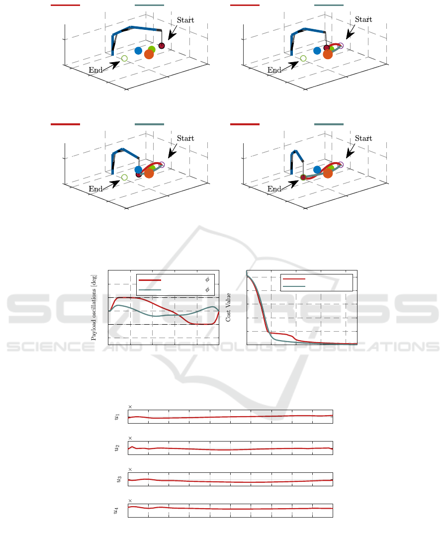
Fig. 2 illustrates the trajectory comparison, where

the green line represents the trajectory without obsta-

cle avoidance and the red line denotes the optimized

trajectory with obstacle avoidance, both trajectories

are generated by DDP method. The crane’s trajectory

without obstacles avoidance collides with the orange

obstacle during its operation. In contrast, the red tra-

jectory, optimized with a relaxed log-barrier function,

successfully generates a feasible trajectory that avoids

all obstacles. This highlights the capability of the DDP

method to eﬀectively plan a collision-free trajectory

in a complex obstacle environment.

Fig. 3 illustrates the payload oscillations during

obstacle avoidance and the corresponding cost opti-

mization over iterations. Fig. 3(a) shows that the

proposed DDP method successfully regulates the pay-

load oscillations in the obstacle avoidance trajectory,

ensuring that they remain within acceptable limits

throughout the entire time horizon and stabilize at

the end. Fig. 3(b) presents the cost evolution for both

scenarios, with and without obstacles. Notably, the

trajectory with obstacles maintains a higher cost due

to the obstacle penalty term, particularly during the

early optimization stages. Ultimately, both scenarios

are converged, demonstrating the eﬀectiveness of the

DDP method in handling obstacle avoidance.

Fig. 4 shows the time evolution of control inputs

from 𝑢

to 𝑢

during the obstacle avoidance process.

The results indicate that the control inputs remain

smooth and within bounds throughout the trajectory.

SIMULTECH 2025 - 15th International Conference on Simulation and Modeling Methodologies, Technologies and Applications

-10

(a)

Z[m]

X[m]

Y[m]

With obstacles Without obstacles

-10

(b)

Z[m]

X[m]

Y[m]

With obstacles Without obstacles

-10

(c)

Z[m]

X[m]

Y[m]

With obstacles Without obstacles

-10

(d)

Z[m]

X[m]

Y[m]

With obstacles Without obstacles

t=0s t=2.7s

t=3.4s t=5s

Figure 2: Trajectory comparison: (a) trajectories at initial instant; (b) trajectories at 2.7s; (c) trajectories at 3.4s; (d) trajectories

at 5s.

0 1 2 3 4 5

Time [s]

-20

-10

(a)

Oscillation angle

0 500 1000 1500 2000

Iteration

200

400

600

800

1000

(b)

With obstacles

Without obstacles

Figure 3: Payload oscillations and cost optimization: (a) payload oscillations during obstacle avoidance; (b) cost evolution

over iterations.

0 0.5 1 1.5 2 2.5 3 3.5 4 4.5 5

-5

0 0.5 1 1.5 2 2.5 3 3.5 4 4.5 5

-1

0 0.5 1 1.5 2 2.5 3 3.5 4 4.5 5

Time [s]

Figure 4: Control inputs during obstacle avoidance: (a) 𝑢

; (b) 𝑢

; (c) 𝑢

; (d) 𝑢

4.3 Comparison of Kinematic

Constraint Violation Suppression

To evaluate the performance of the DDP method in

suppressing kinematic constraint violations, which is

achieved by applying a Baumgarte stabilization ap-

proach within the transformed dynamics, this section

compares its results with those of the Ipopt solver that

directly solves the dynamics described in Eq. (2).

This case involves a spherical obstacle with a radius

Trajectory Planning for a Knuckle Boom Crane Using Differential Dynamic Programming

-10

(a)

Z[m]

X[m]

Y[m]

DDP Ipopt

-10

(b)

Z[m]

X[m]

Y[m]

DDP Ipopt

-10

(c)

Z[m]

X[m]

Y[m]

DDP Ipopt

-10

(d)

Z[m]

X[m]

Y[m]

DDP Ipopt

t=0s t=2.7s

t=3.4s t=5s

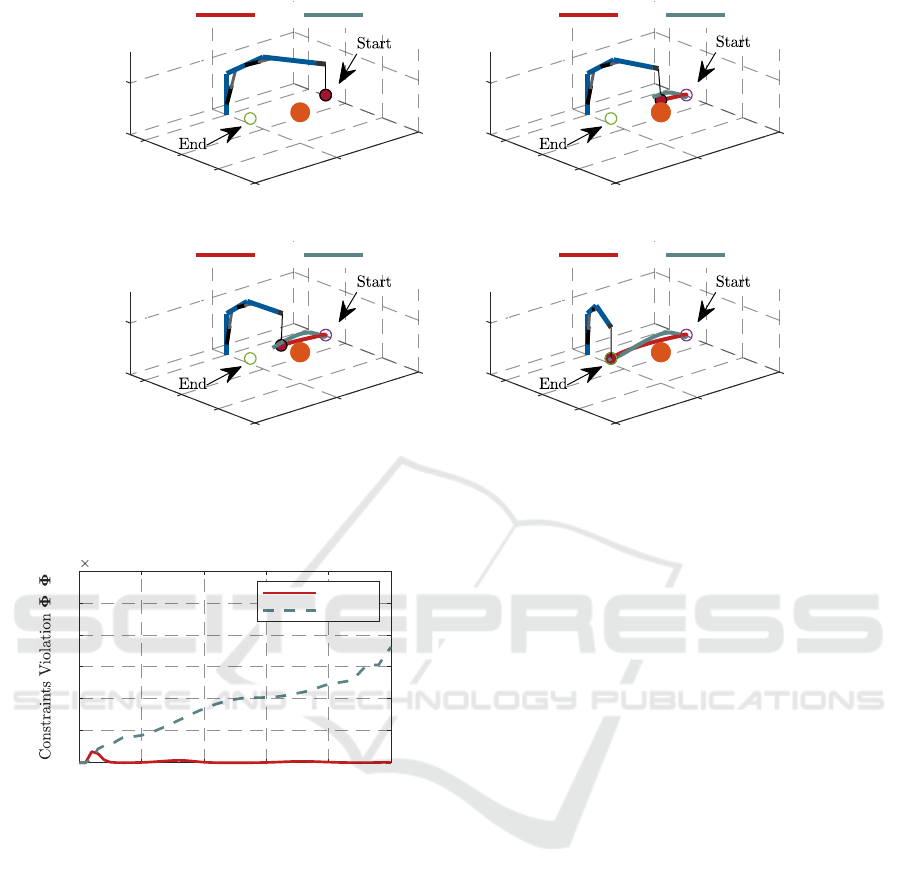
Figure 5: Trajectory comparison of the two solvers: (a) trajectories at initial instant; (b) trajectories at 2.7s; (c) trajectories at

3.4s; (d) trajectories at 5s.

0 1 2 3 4 5

Time [s]

0.5

1.5

2.5

-7

Proposed

Ipopt

Figure 6: Kinematic constraints violation comparison.

of 1m, positioned at 𝑝

𝑝

= (0, 10, 3). All other param-

eters remain the same as in Subsection 4.2. To balance

convergence speed and accuracy, Ipopt’s convergence

tolerance is set to 1 × 10

−6

. In this case, the violation

error 𝚽

⊤

𝚽 is used to evaluate each method’s perfor-

mance in suppressing kinematic constraint violations.

Fig. 5 presents the optimization results obtained

by the two solvers. The results indicate that both the

proposed method and Ipopt generate feasible obstacle

avoidance trajectories.

Fig. 6 compares the constraint violation suppres-

sion performance between the DDP method with the

transformed crane dynamics and the Ipopt solver. The

results show that the constraint violation for the Ipopt

solver increases over time. In contrast, the DDP

method with the transformed crane dynamics main-

tains a low and stable constraint violation throughout

the entire time horizon. This diﬀerence indicates that

Baumgarte stabilization eﬀectively prevents the accu-

mulation of constraint errors in the dynamic system.

5 CONCLUSIONS

In this paper, we investigated an obstacle avoidance

trajectory planning method for knuckle boom cranes.

The standard Lagrange multiplier method, combined

with Baumgarte stabilization, was employed to de-

rive the crane’s dynamic equations, which were then

expressed in an explicit Euler form to facilitate the

design of the DDP method. In addition, we adopted a

relaxed log-barrier function to handle state constraints

and obstacle avoidance during crane operation. The

eﬀectiveness of the proposed approach was validated

through simulations in MATLAB, where the kine-

matic constraint suppression performance was com-

pared with the Ipopt solver. The results demonstrated

the advantages of the proposed method for trajectory

planning in kinematically constrained mechanical sys-

tems.

ACKNOWLEDGEMENTS

This research was funded by the China Scholarship

Council (Grant No. 202109150003).

SIMULTECH 2025 - 15th International Conference on Simulation and Modeling Methodologies, Technologies and Applications

REFERENCES

Andersson, J. A. E., Gillis, J., Horn, G., Rawlings, J. B., and

Diehl, M. (2019). CasADi – A software framework

for nonlinear optimization and optimal control. Math-

ematical Programming Computation, 11(1):1–36.

Aoyama, Y., Boutselis, G., Patel, A., and et al. (2021). Con-

strained diﬀerential dynamic programming revisited.

In 2021 IEEE International Conference on Robotics

and Automation (ICRA), pages 9738–9744. IEEE.

Chen, J., Zhan, W., and Tomizuka, M. (2019). Autonomous

driving motion planning with constrained iterative lqr.

IEEE Transactions on Intelligent Vehicles, 4(2):244–

254.

Farrage, A., Takahashi, H., Terauchi, K., and et al. (2023).

Trajectory generation of rotary cranes based on a* al-

gorithm and time-optimization for obstacle avoidance

and load-sway suppression. Mechatronics, 94:103025.

Grandia, R., Farshidian, F., Ranftl, R., and et al. (2019).

Feedback mpc for torque-controlled legged robots. In

2019 IEEE/RSJ International Conference on Intelli-

gent Robots and Systems (IROS), pages 4730–4737.

IEEE.

Huang, Z., Shen, S., and Ma, J. (2023). Decentralized

ilqr for cooperative trajectory planning of connected

autonomous vehicles via dual consensus admm. IEEE

Transactions on Intelligent Transportation Systems.

Jallet, W., Bambade, A., Mansard, N., and et al. (2022).

Constrained diﬀerential dynamic programming: A

primal-dual augmented lagrangian approach. In

2022 IEEE/RSJ International Conference on Intelli-

gent Robots and Systems (IROS), pages 13371–13378.

IEEE.

Kazdadi, S. E., Carpentier, J., and Ponce, J. (2021). Equal-

ity constrained diﬀerential dynamic programming. In

2021 IEEE International Conference on Robotics and

Automation (ICRA), pages 8053–8059. IEEE.

Kim, G., Kang, D., Kim, J. H., and et al. (2022). Contact-

implicit diﬀerential dynamic programming for model

predictive control with relaxed complementarity con-

straints. In 2022 IEEE/RSJ International Confer-

ence on Intelligent Robots and Systems (IROS), pages

11978–11985. IEEE.

Lee, Y., Cho, M., and Kim, K. S. (2022). Gpu-parallelized

iterative lqr with input constraints for fast collision

avoidance of autonomous vehicles. In 2022 IEEE/RSJ

International Conference on Intelligent Robots and

Systems (IROS), pages 4797–4804. IEEE.

Li, G., Ma, X., Li, Z., and et al. (2022). Optimal tra-

jectory planning strategy for underactuated overhead

crane with pendulum-sloshing dynamics and full-state

constraints. Nonlinear Dynamics, 109(2):815–835.

Li, H. and Wensing, P. M. (2020). Hybrid systems diﬀer-

ential dynamic programming for whole-body motion

planning of legged robots. IEEE Robotics and Au-

tomation Letters, 5(4):5448–5455.

Marques, F., Souto, A. P., and Flores, P. (2017). On the

constraints violation in forward dynamics of multibody

systems. Multibody System Dynamics, 39:385–419.

Martin, I. A. and Irani, R. A. (2021). Dynamic modeling

and self-tuning anti-sway control of a seven degree of

freedom shipboard knuckle boom crane. Mechanical

Systems and Signal Processing, 153:107441.

Mastalli, C., Budhiraja, R., Merkt, W., and et al. (2020).

Crocoddyl: An eﬃcient and versatile framework for

multi-contact optimal control. In 2020 IEEE In-

ternational Conference on Robotics and Automation

(ICRA), pages 2536–2542. IEEE.

Thi, H. L., Vu, M. N., Khanh, H. B. T., and et al. (2024).

Flatness-based motion planning and control strategy

for payload positioning of an overhead crane.

Wang, Y., Li, H., Zhao, Y., and et al. (2023). A fast co-

ordinated motion planning method for dual-arm robot

based on parallel constrained ddp. IEEE/ASME Trans-

actions on Mechatronics.

Zhang, W., Chen, H., Chen, H., and et al. (2021). A time op-

timal trajectory planning method for double-pendulum

crane systems with obstacle avoidance. IEEE Access,

9:13022–13030.

Zheng, X., He, S., and Lin, D. (2021). Constrained tra-

jectory optimization with ﬂexible ﬁnal time for au-

tonomous vehicles. IEEE Transactions on Aerospace

and Electronic Systems, 58(3):1818–1829.

Zhu, H., Ouyang, H., and Xi, H. (2023). Neural network-

based time optimal trajectory planning method for ro-

tary cranes with obstacle avoidance. Mechanical Sys-

tems and Signal Processing, 185:109777.

Zimmermann, S., Poranne, R., and Coros, S. (2021). Dy-

namic manipulation of deformable objects with im-

plicit integration. IEEE Robotics and Automation Let-

ters, 6(2):4209–4216.

Trajectory Planning for a Knuckle Boom Crane Using Differential Dynamic Programming