eXplainable Artiﬁcial Intelligence Framework for Structure’s Limit

Load Extimation

Habib Imani

3 a

, Renato Zona

1 b

, Armando Arcieri

, Luigi Piero Di Bonito

2 c

Simone Palladino

1 d

and Vincenzo Minutolo

1 e

Department of Engineering, Universit

a della Campania Vanvitelli,Via Roma 29, Aversa (CE), Italy

Dipartimento di Ingegneria Chimica, dei Materiali e della Produzione Industriale, Universit

a degli Studi di Napoli

”Federico II”, Naples, Italy

Department of Engineering and Architecture, Universit

a degli Studi di Catania,Via S.Soﬁa 64, Catania (CT), Italy

Independent Researcher, Italy

Keywords:

Machine Learning, Finite Element, Limit Analysis, Virtual Twin, Vulnerability.

Abstract:

The recent advancements in machine learning (ML) and deep learning (DL) have signiﬁcantly expanded op-

portunities across various ﬁelds. While ML is a powerful tool applicable to numerous disciplines, its direct

implementation in civil engineering poses challenges. ML models often fail to perform reliably in real-world

scenarios due to lack of transparency and explainability during the decision-making process of the algorithm.

To address this, physics-based ML models integrate data obtained through a ﬁnite element procedure based on

the lower bound theorem of limit analysis, ensuring compliance with physical laws described by general non-

linear equations. These models are designed to handle supervised learning tasks while mitigating the effects

of data shift. Widely recognized for their applications in disciplines such as ﬂuid dynamics, quantum me-

chanics, computational resources, and data storage, physics-based ML is increasingly being explored in civil

engineering. In this work, a novel methodology that combines machine learning and computational mechanics

to evaluate the seismic vulnerability of existing buildings is proposed. Interesting and affordable results are

reported in the paper concerning the predictability of limit load of structure through ML approaches. The aim

is to provide a practical tool for professionals, enabling efﬁcient maintenance of the built environment and

facilitating the organization of interventions in response to natural disasters such as earthquakes.

1 INTRODUCTION

Machine Learning (ML) and Deep Learning (DL),

such as deep neural networks (DNNs), are increas-

ingly integrated into the scientiﬁc process, replacing

traditional statistical methods and mechanistic models

across various sectors and ﬁelds, including education

(Momeny et al., 2021), natural and environmental sci-

ences (Malami et al., 2021; Campanile et al., 2024),

medicine (Sharma et al., 2021; Vadyala and Sherer,

2021), engineering (Santhosh et al., 2021; Campanile

et al., 2023; Di Bonito et al., 2023), and social sci-

ences (Ciaccio and Troisi, 2021). In civil engineer-

https://orcid.org/0009-0004-6455-3779

https://orcid.org/0000-0001-6718-9387

https://orcid.org/0000-0001-5002-4789

https://orcid.org/0000-0001-6718-9387

https://orcid.org/0000-0002-7787-4844

ing, where mechanistic models have historically pre-

vailed, ML is also gaining traction (Vadyala et al.,

2021, 2022). Despite its growing adoption, ML meth-

ods are often criticized by researchers and end users

as a ”black box,” as they provide inputs and outputs

without offering physically interpretable insights to

the user (McGovern et al., 2019). This critique has

driven some scientists to eXplainable Artiﬁcial Intel-

ligence (XAI) models to address concerns regarding

the opacity of black-box methods (Gunning and Aha,

2019; Alber et al., 2019; Laub, 1999; Karpatne et al.,

2017). In civil engineering, ML models are generated

directly from data through algorithms, yet even their

developers often struggle to fully understand how in-

put variables are combined to produce predictions.

While these models identify relevant input variables,

their complexity makes it difﬁcult to discern the in-

teractions that lead to ﬁnal predictions. In this con-

Imani, H., Zona, R., Arcieri, A., Piero Di Bonito, L., Palladino, S. and Minutolo, V.

eXplainable Artiﬁcial Intelligence Framework for Structure’s Limit Load Extimation.

DOI: 10.5220/0013519800003944

In Proceedings of the 10th International Conference on Internet of Things, Big Data and Security (IoTBDS 2025), pages 469-480

ISBN: 978-989-758-750-4; ISSN: 2184-4976

469

text, the development of XAI plays a crucial role in

improving the trustworthiness and robustness of both

ML and DL models, particularly for critical applica-

tions where safety is a key concern (Di Bonito et al.,

2024). For instance, ML models that fail to accu-

rately estimate structural damage are often associated

with processes that are not entirely understood and

present challenges such as high data requirements,

difﬁculty in providing physically consistent ﬁndings,

and limited generalizability to out-of-sample scenar-

ios. Large, curated datasets with well-deﬁned, pre-

cisely labeled categories are typically used to evaluate

ML and DL models (Momeny et al., 2021). While DL

performs well under such conditions, it assumes a rel-

atively stable environment. The environment bound-

ary conditions are taken into account. Soil structure

interaction is a future perspective to be considered.

Recent developments in soil identiﬁcation (Damiano

et al., 2024; de Cristofaro et al., 2024) suggest to con-

sider the soil as a detailed boundary condition. In this

paper a well-established procedure (Zona and Minu-

tolo, 2024) was used to construct a reference database

for the limit load assessment of frame structures. The

aim was to obtain an initial approach to the calcula-

tion based on post-hoc XAI methodology (Barredo

Arrieta et al., 2020) to assess the reliability of the

results when varying various predeﬁned parametric

conditions.

2 FROM FINITE ELEMENT

LIMIT ANALYSIS TO

MACHINE LEARNING

This paper introduces a methodology to determine

the limit load of civil structures under standard load-

ing conditions. The objective is to develop a tool

that surpasses conventional approaches to assess the

ultimate strength of structures. A detailed descrip-

tion of an alternative computational procedure, differ-

ent from those outlined in current standards, is pro-

vided in Mangalathu et al. (2020). The advancement

of this methodology lies in the use of the limit load

as a parameterized indicator of seismic vulnerability.

The shift from traditional computational mechanics

to Computational Mechanics 3.0 is facilitated through

the application of machine learning algorithms. These

algorithms enable the generation of reliable and ac-

tionable results for managing seismic emergency sce-

narios in a signiﬁcantly shorter timeframe compared

to classical computational methods. The seismic

risk classiﬁcation for individual buildings—critical

for predicting potential earthquake impacts—relies on

structural resistance characteristics derived from ge-

ometry and material properties. This process estab-

lishes qualitative assessment criteria through site in-

spections and surveys, factoring in building typology,

construction date, and the regulations in effect dur-

ing the building’s erection. These criteria help extract

quantitative data on mechanical properties, which can

then be applied to simpliﬁed analytical models.

The conducted surveys aim to develop representa-

tive numerical models that enable rapid and reliable

assessments of structural resistance and vulnerabil-

ity. At the building scale, structural characterization

is achieved by analyzing and categorizing settlements

into homogeneous groups based on the following pa-

rameters:

• Geometric conﬁguration

• Construction date (age of the structure and build-

ing methods)

• Regulatory framework at the time of construction,

providing insights at the broader building sector

level

• Neighborhood context and its inﬂuence on ex-

pected vulnerability

This data supports the creation of a numerical twin for

each building type (morphotype), allowing the iden-

tiﬁcation of zones with comparable risk parameters.

Consequently, seismic micro-zoning can be imple-

mented, focusing on structural vulnerabilities. By ap-

plying micro-zoning at a micro-seismic scale, it be-

comes possible to assess earthquake effects through

qualitative and topological classiﬁcations of building

vulnerabilities, considering both existing damage and

potential future risks. Ultimately, the goal is to de-

velop simpliﬁed strategies for evaluating and analyz-

ing structural performance. These strategies rely on

indirect assessments, enabling the interpretation of

a building’s structural behavior through quantitative

parameters derived from observations and simpliﬁed

measurements across building clusters.

2.1 Finite Element Limit Analysis via

VFEM Methodology

This analytical approach employs a static limit anal-

ysis framework implemented through specialized ﬁ-

nite element procedures. The method establishes the

mathematical foundation for self-equilibrated stress

ﬁelds (Zona et al., 2021) through linear optimiza-

tion techniques (VFEM protocol) (Zona and Minu-

tolo, 2024). The formulation originates from Volterra

dislocation theory, utilizing isoparametric shape func-

tions that map discontinuous displacement ﬁelds

through nodal parameters.

AI4EIoT 2025 - Special Session on Artiﬁcial Intelligence for Emerging IoT Systems: Open Challenges and Novel Perspectives

470

The computational core implements an optimiza-

tion routine that determines the critical load mul-

tiplier by evaluating statically admissible solutions,

with Melan residuals expressed as nodal disloca-

tion parameters. The stress-strain relationship de-

rives from strain representations generated through

shape function derivatives, accommodating various

structural models through adaptable element formu-

lations. Displacement-based nodal parameters simul-

taneously characterize internal dislocation patterns,

creating a uniﬁed FEM framework that links self-

equilibrated stresses to nodal variables. This formula-

tion enables direct limit load calculation through con-

strained optimization:

= sup

k, | (kσ

∗

+ V δ) ∈ D

α =

(

sd, shakedown

c, collapse

(1)

where the eigenstress ﬁeld emerges from the nodal

mapping (1):

= V δ (2)

The singular matrix V relates element stress vec-

tors to nodal parameters δ. This methodology

eliminates conventional limitations requiring detailed

load history knowledge, particularly advantageous for

structures subjected to stochastic loading scenarios.

Melan’s approach proves robust against load path

uncertainties, focusing instead on critical load pat-

terns and intensity domains. The framework enables

comprehensive safety assessment through parametric

studies across structural morphotypes. Key vulnera-

bility indicators include:

• Span conﬁgurations in principal directions

• Vertical height-to-span ratios

• Relative strength of vertical vs. horizontal mem-

bers

Through a comprehensive computational approach,

the structural safety level can be estimated based on

both load and displacement parameters. This method-

ology involves a parametric analysis of numerous nu-

merical experiments conducted on various structural

types, leading to the development of risk abacuses.

The procedure encompasses modeling structures with

diverse morphological and topological characteris-

tics while thoroughly examining their structural re-

sponses. For each structural morpho-type, the capac-

ity curve is deﬁned based on its key parameters. The

safety factor for each morpho-type is then precisely

determined based on inﬂuential parameters such as

the number of spans in the primary structural layout

directions, the overall height, and the strength ratios

of columns and beams. The key parameters char-

acterizing the capacity curve—safety factor, ultimate

displacement at collapse, and residual displacements

related to residual stresses—allow for direct compar-

isons among different morpho-types. This compar-

ative analysis facilitates the assessment of structural

vulnerability across various building groups.

2.2 Finite Element Limit Analysis

(FELA) Formulation

A stress ﬁeld, σ

, is considered statically admissible

if it satisﬁes the equilibrium conditions while remain-

ing conﬁned within the domain D

= (σ

∗

+ σ

) ∈



∩



(3)

The Greenberg-Prager lower bound theorem in limit

analysis states that a load in equilibrium with a stat-

ically admissible stress does not result in structural

collapse. Furthermore, if the material adheres to

the Drucker stability condition and the load can be

expressed using a multiplicative factor k such that

σ(t) = kσ

∗

(t) + σ

(t), then the ultimate load corre-

sponds to the supremum of k.

Several important phenomena are encompassed in

this description. Speciﬁcally, when a unique load pat-

tern is applied and the multiplier k serves as a mono-

tonically increasing parameter, the supremum of k de-

ﬁnes the collapse threshold. Beyond this straightfor-

ward case, when a structure experiences multiple load

patterns whose intensities can be bounded by a com-

mon scalar factor k, additional failure mechanisms

such as shakedown, ratcheting, and low-cycle fatigue

must also be considered, provided that the stress en-

velope throughout the structure’s time history is prop-

erly accounted for.

In all scenarios, determining the load limit reduces

to solving an optimization problem in terms of the

time-independent eigenstress ¯σ

, as summarized in

the following equation:

{

sup

(kσ

∗

+ ¯σ

) ∈ D

}

α =



sd shakedown

c collapse

(4)

Deﬁning a discretized form of the eigenstress domain,

where the solution is to be sought, is essential for

determining the load limit using the ﬁnite element

method (FEM).

The formulation adopted in this study, as pre-

sented in Zona and Minutolo (2024), expresses eigen-

stress in terms of a set of nodal parameters δ, which

represent eigenstrain as a dislocation distribution

within the elements.

= V δ (5)

eXplainable Artiﬁcial Intelligence Framework for Structure’s Limit Load Extimation

471

Based on equation (5), if there exists a nodal param-

eter set

δ that ensures the stress remains within the

elastic domain at every stage of the load path, the

structure avoids an unbounded accumulation of plas-

tic strain. Consequently, failure due to collapse, alter-

nating plasticity, or ratcheting does not occur.

The load limit multiplier is obtained as the supre-

mum of the load multipliers in the constrained opti-

mization problem (4), modiﬁed according to equation

(5), as follows:

= sup

(kσ

∗

+ V δ) ∈ D

α =



sd shakedown

c collapse

(6)

The matrix V is singular, with two dimensions corre-

sponding to the size of the element stress vector and

δ, respectively. The rank of V represents the number

of independent solutions to the equilibrium equations

and aligns with the structural redundancies. In trusses

and frames, this rank is ﬁnite and independent of dis-

cretization, whereas for other structural systems, it is

inherently inﬁnite. When discretization is applied, the

rank becomes ﬁnite and depends on the chosen dis-

cretization scheme. However, in general, the rank of

V remains lower than its total dimensions.

Different constitutive models deﬁne distinct do-

mains, which impose constraints on the optimiza-

tion procedure. The constraint inequalities utilized

in the calculations have been linearized by approxi-

mating the domain with an inscribed polyhedron. In

the case of plane stress conditions, this linearized do-

main forms an octahedron that matches the nonlinear

domain at its intersections with the coordinate axes,

leading to the following set of linear inequalities:

∑

∏

j−{i}

jlβ

≤

∏

jlβ

(7)

The expression in (7) consists of f inequality con-

straints, where r = {1, ..., f }, positioned at the faces

of the polyhedron. For an octahedral domain under

plane stress conditions, f = 8. These constraints (7)

are applied at the nodal points of the ﬁnite element

model. Given that the actual stress σ

has been de-

composed according to equation (5), the optimiza-

tion problem is reformulated as a linear programming

problem:

sup



∑

∏

j−{i}

jlβ

(kσ

∗

− V δ)

≤

∏

jlβ

(8)

When the applied loads are divided into a constant

dead load and a live load that can increase with a mul-

tiplier k, the stress is split into a ﬁxed part σ

and a

variable part kσ

. The stress representation is then

modiﬁed as:

σ = σ

+ kσ

+ V δ

Consequently, the compatibility inequalities are trans-

formed to:

sup



∑

∏

j\{i}

jlβ



kσ

h∗

+ V δ + σ

p∗





≤ α

∏

j=1

jlβ

The solutions obtained from the optimization pro-

grams in (8) provide the load multiplier at the collapse

or shakedown limit.

In the present analysis, the ﬁnite element dis-

cretization is composed of two-dimensional isopara-

metric 4-node linear elements. The input rou-

tines were generated using the Ansys© preproces-

sor macro, which produced database ﬁles contain-

ing node coordinates, element connectivity, material

properties, and applied loads. This data was subse-

quently processed within a custom procedure for limit

analysis. The developed routine assembled the re-

quired matrices, computed the elastic stress state, for-

mulated the constraints for the optimization problem,

and determined the ultimate load multiplier through

an optimization-based approach.

The geometric interpretation of the compatibil-

ity constraints is illustrated in Figure 1. It can be

observed that employing a linearized domain results

in a conservative estimate of the structural strength.

To mitigate this underestimation, a correction factor

is introduced. As discussed in (Zona and Minutolo,

2024) and demonstrated in Figure 2, an ampliﬁca-

tion factor is applied along the actual stress trajec-

tory. This factor corresponds to the ratio between the

distance from the origin to the plane parallel to the

polyhedral face, where the extended stress vector in-

tersects the nonlinear domain, and the corresponding

linearized polyhedral face, as depicted in Figures 1

and 2.

Figure 1: Linearized limit domain inscribed in the ellipsoid.

α =

> 1 (9)

AI4EIoT 2025 - Special Session on Artiﬁcial Intelligence for Emerging IoT Systems: Open Challenges and Novel Perspectives

472

Figure 2: Geometric representation of the α factor.

2.3 Database Construction

For performing linear static analysis on the frames,

the VFEM routine was utilized. The procedure fol-

lows a structured approach: initially, the frame model

is developed using FEM software, which serves ex-

clusively as a CAD interpreter. This method simpli-

ﬁes the speciﬁcation of nodal connectivity, element

types, and boundary conditions. Additionally, an au-

tomated routine was implemented to generate vari-

ous frame conﬁgurations, which are subsequently an-

alyzed and compiled into a results table that forms the

basis of the vulnerability assessment.

The FELA routine computes the load multiplier

at the elastic limit, the collapse load multiplier, and

the maximum elastic displacements. These results are

systematically stored in a tensor, encapsulating data

for each morphological frame type. The overall work-

ﬂow is illustrated in Figure 5.

A CAD compiler enables an automated proce-

dure for evaluating various structural conﬁgurations.

Speciﬁcally, a series of structures is generated with

different numbers of ﬂoors, columns, and column

spacing. The output ﬁlename of each frame encodes

its corresponding geometric characteristics:

VirtualTWIN

i− j−h−k−l−m

(10)

i → number of pillars in the x direction

j → number of pillars in the z direction

h → number of ﬂoors in the y direction

k = 3 → distance between each ﬂoor

l → distance between pillars in x direction

m → distance between pillars in z direction

An essential parameter in virtual twin modeling is

the cross-sectional dimensions of beams and columns.

In this study, a cross-section of 60 × 40 cm is adopted.

The collapse multiplier results are obtained by

considering the specialized limit domain. To com-

pute the collapse multiplier, an optimization routine

Figure 3: VirtualTWIN: i=4, j=4, h=2, k=3, l=m=4.

Figure 4: VirtualTWIN with (60x40) cm cross-section.

based on linear programming is employed, solving a

constrained optimization problem with a linear objec-

tive function and linear constraints. In the present

case, the constraints are deﬁned by the boundary of

the limit domain, while the objective function corre-

sponds to the collapse multiplier.

For the application of linear programming, the

plastic compatibility domain of a generic beam sec-

tion under biaxial bending, characterized by three

stress components, is linearized using a ﬂat-plane ap-

proximation. Speciﬁcally, eight planes, each corre-

sponding to one of the faces of a non-regular octa-

hedron tangential to the curved domain, are utilized.

Although the domain can be enveloped with multi-

ple ﬂat layers without compromising the algorithm’s

fundamental properties, this approach introduces ad-

ditional computational complexity.

Consequently, the boundary polyhedron faces are

characterized by six distinct boundary stress val-

ues: M

ytu

, M

ycu

, M

ztu

, M

zcu

, N

. The subscripts of

eXplainable Artiﬁcial Intelligence Framework for Structure’s Limit Load Extimation

473

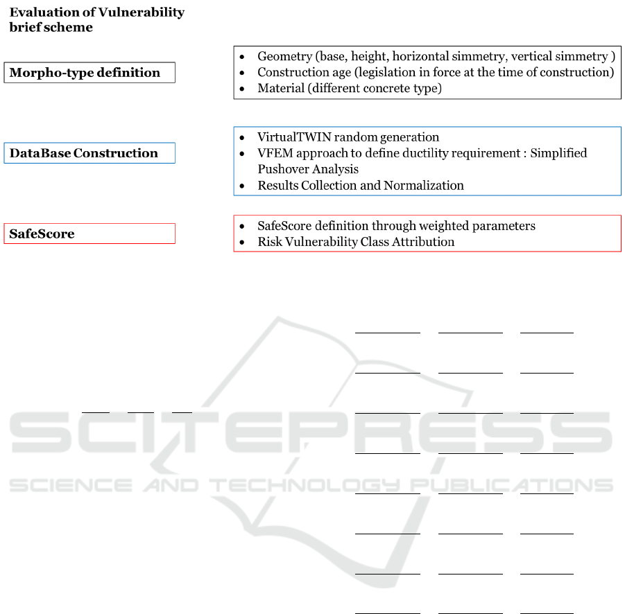
Figure 5: Procedure Workﬂow.

these stresses denote the direction of the acting mo-

ments (y or z) and whether the stress corresponds to

tension or compression (t/c) based on the positive or

negative intersection with the respective axis. This

formulation allows the planes of the octahedron to be

represented through the following equations:

yβu

zβu

βu

= 1 (11)

where β = t or c, and the quantities in the denomina-

tor take the values speciﬁed above, while the terms in

the numerator represent the stresses obtained from the

structural analysis.

The generic stress can be formulated as a com-

bination of the corresponding components of V and

the ampliﬁed elastic rate associated with an arbitrary

multiplier k.

δ+kM

, M

δ+kM

, N =V

δ+kN

(12)

The previously mentioned positions, when substi-

tuted into the equation 11, offer a representation based

on stress parameters. Being part of the internal limit

domain of the loading is equivalent to fulﬁlling the

inequalities of the linearized domain, which are ex-

pressed by the following eight matrix inequalities in

terms of δ and k.

The optimization problem associated with the

static theorem (in Melan’s form) involves ﬁnding the

maximum value of k subject to the following con-

straints:



δ + kM

ytu

δ + kM

ztu

δ + kN



< 1



δ + kM

ycu

δ + kM

ztu

δ + kN



< 1



δ + kM

ytu

δ + kM

zcu

δ + kN



< 1



δ + kM

ycu

δ + kM

ztu

δ + kN



< 1



δ + kM

ytu

δ + kM

zcu

δ + kN



< 1



δ + kM

ycu

δ + kM

ztu

δ + kN



< 1



δ + kM

ycu

δ + kM

zcu

δ + kN



< 1



δ + kM

ycu

δ + kM

zcu

δ + kN



< 1

(13)

The procedure was implemented on a dataset con-

sisting of 405 distinct structural morpho-types. The

outcomes are presented in terms of SafeScore (SS),

calculated as shown in Eq. (14):

SS = α · β · γ · δ · η · ζ · S

cV FEM

(14)

The parameter S

cV FEM

represent the collapse multi-

plier for each load case. In the case, the results are

reported for the Permanent Load (self weight + addi-

tional load) and Seismic X and Seismic Z load. The

AI4EIoT 2025 - Special Session on Artiﬁcial Intelligence for Emerging IoT Systems: Open Challenges and Novel Perspectives

474

coefﬁcients of the S

cV FEM

represents respectively:

α = base regularity

β = height regularity

γ = base − height ratio

δ = age o f costruction

η = cross − section

ζ = material

The initial set of results is presented in terms of elas-

tic limit load, SE

, collapse limit load, SC

, and the

ratio between SE and SC, denoted as R

, where the

subscript i = {1,2, 3} is deﬁned as:











i = 1 gravity load

i = 2 seismic load in x direction

i = 3 seismic load in z direction

The objective is to enhance the calculation method-

ology by integrating the most advanced techniques in

Machine Learning and deep learning, using the struc-

tured database described. The database incorporates

input data for 405 frames:

• number of pillars in the two plane directions

• number of ﬂoors

• ultimate bending moments

• ultimate normal stress resistance

• section of the beams

• Area

• Inertia

The anticipated output is the limit resistance of the

structures under various loading conditions, speciﬁ-

cally vertical load simulating self weight of the struc-

ture and seismic load.

3 eXplainable ARTIFICIAL

INTELLIGENCE

3.1 Dataset Description

The initial phase involved understanding the charac-

teristics of the dataset attributes. Table 3 summarizes

the features of the dataset, and Table 1 and 2 contains

the descriptive statistics of the dataset.

For the comprehensive dataset analysis, the data

examination predominantly relied on Python pro-

gramming language and the Pandas library within the

Jupyter Notebook environment.

Table 1: Descriptive Statistics of the Dataset.

Count Mean Std Min

nx 404.0000 4.0025 0.8170 3.0000

ny 404.0000 3.9975 1.4168 2.0000

nz 404.0000 4.0025 0.8170 3.0000

lx 404.0000 5.0000 0.8185 4.0000

lz 404.0000 4.9975 0.8170 4.0000

Peso 404.0000 12000.0000 0.0000 12000.0000

404.0000 577258.6634 209408.7459 288000.0000

404.0000 57725.8663 20940.8746 28800.0000

404.0000 576924.5049 209143.9775 288000.0000

404.0000 57692.4505 20914.3978 28800.0000

404.0000 2698663.3663 628660.3943 1728000.0000

404.0000 128279.7030 46535.2769 64000.0000

T PIANO 404.0000 1265.1609 425.0504 533.0000

404.0000 45495.6683 22821.3029 9600.0000

404.0000 0.4000 0.0000 0.4000

404.0000 0.6000 0.0000 0.6000

404.0000 0.4000 0.0000 0.4000

404.0000 0.6000 0.0000 0.6000

404.0000 0.2400 0.0000 0.2400

404.0000 0.3600 0.0000 0.3600

404.0000 0.0072 0.0000 0.0072

404.0000 0.0032 0.0000 0.0032

404.0000 0.0108 0.0000 0.0108

EM Permanent load 404.0000 3.8505 0.1954 3.2168

EM Seismic x 404.0000 2.2121 0.4707 1.2191

EM Seismic y 404.0000 2.2177 0.4528 1.2285

CM Permanent load 404.0000 5.9839 0.1660 5.4500

CM Seismic x 404.0000 2.8534 0.5882 0.0000

CM Seismic y 404.0000 2.7108 0.7671 0.0000

Table 2: Descriptive Statistics of the Dataset.

25% 50% 75% Max

nx 3.0000 4.0000 5.0000 5.0000

ny 3.0000 4.0000 5.0000 6.0000

nz 3.0000 4.0000 5.0000 5.0000

lx 4.0000 5.0000 6.0000 6.0000

lz 4.0000 5.0000 6.0000 6.0000

Peso 12000.0000 12000.0000 12000.0000 12000.0000

432000.0000 562500.0000 675000.0000 972000.0000

43200.0000 56250.0000 67500.0000 97200.0000

432000.0000 562500.0000 675000.0000 972000.0000

43200.0000 56250.0000 67500.0000 97200.0000

2160000.0000 2592000.0000 3240000.0000 3888000.0000

96000.0000 125000.0000 150000.0000 216000.0000

T PIANO 960.0000 1200.0000 1500.0000 2700.0000

27000.0000 43200.0000 56250.0000 145800.0000

0.4000 0.4000 0.4000 0.4000

0.6000 0.6000 0.6000 0.6000

0.4000 0.4000 0.4000 0.4000

0.6000 0.6000 0.6000 0.6000

0.2400 0.2400 0.2400 0.2400

0.3600 0.3600 0.3600 0.3600

0.0072 0.0072 0.0072 0.0072

0.0032 0.0032 0.0032 0.0032

0.0108 0.0108 0.0108 0.0108

EM Permanent load 3.7808 3.9197 3.9834 4.0642

EM Seismic x 1.9884 2.3095 2.5811 3.0471

EM Seismic y 1.9089 2.2929 2.5629 3.0413

CM Permanent load 5.9344 5.9736 6.1234 6.6315

CM Seismic x 2.5756 2.8951 3.3021 3.8555

CM Seismic y 2.0464 2.9081 3.3994 3.9177

3.2 Evaluation Metrics

To assess the predictive capability of the regres-

sion model for the feature CM Permanent load, the

dataset was partitioned into 70% for training and 30%

for testing. The evaluation of the model’s accuracy in-

volved computing the Mean Square Error (MSE) Eq.

(15), Mean Absolute Error (MAE) Eq. (16), and the

Coefﬁcient of Determination (R

) Eq. (17).

MSE(y,

y) =

n−1

∑

i=0

−

)

(15)

eXplainable Artiﬁcial Intelligence Framework for Structure’s Limit Load Extimation

475

Table 3: Dataset features.

Features Unit Description

nx m numbero f pillarsinxdirection

nplane

ny m numbero f pillarsinydirection

uto f plane

nz m numbero f pillarsinzdirection

nplane

lx m spanlengthinxdirection

lz m spanlengthinzdirection

Peso N Sel f weighto f thestructure

M21 Nm limitbendingmoment

M31 Nm limitbendingmoment

M22 Nm limitbendingmoment

M32 Nm limitbendingmoment

N3 N limitnormalstress

N12 N limitnormalstress

T PIANO N Shearplanestress

M3 Nm limitbendingmoment

H1 m sectionedgelength

B1 m sectionedgelength

H2 m sectionedgelength

B2 m sectionedgelength

H3 m sectionedgelength

B3 m sectionedgelength

A1 m

sectionarea

A2 m

sectionarea

A3 m

sectionarea

I1 m

SectionInertia

I2 m

SectionInertia

I3 m

SectionInertia

EM Permanent load / elasticsel f weightymultiplier

EM Seismic x / elasticseismicxmultiplier

EM Seismic y / elasticseismiczmultiplier

CM Permanent load / plasticsel f weightymultiplier

CM Seismic x / plasticseismicxmultiplier

CM Seismic y / plasticseismiczmultiplier

MAE(y,

y) =

n−1

∑

i=0

−

| (16)

(y,

y) = 1 −

∑

i=0

−

)

∑

i=0

− ¯y

)

(17)

where:

• y

denotes the predicted value;

•

represents the observed value;

• ¯y

∑

k=1

corresponds to the mean of the ac-

tual values.

The MAE and MSE metrics quantify the average ab-

solute deviation and the squared deviation of pre-

dictions, respectively, while R

indicates the propor-

tion of variance explained by the model, providing an

overall measure of its goodness of ﬁt.

3.3 Feature Engineering

The selection of representative features is crucial for

the performance and generalization of AI models. To

prevent overﬁtting and underﬁtting, a feature reduc-

tion process is applied before model implementation

(Domingos, 2012; Guyon and Elisseeff, 2003). Vari-

ous techniques exist for this purpose, including Prin-

cipal Component Analysis (PCA), Linear Discrimi-

nant Analysis (LDA), and Pearson correlation anal-

ysis (Velliangiri et al., 2019). In this study, Pearson

correlation was employed to identify the most rele-

vant feature set by measuring the linear association

between variables. Features with a correlation coef-

ﬁcient above a deﬁned threshold (e.g. σ

≥ 0.85)

were removed to reduce redundancy while preserv-

ing model interpretability and robustness (Pearson,

1895).

The Pearson correlation coefﬁcient is deﬁned as:

cov(x, y)

(18)

where cov(x, y) represents the covariance between

variables x and y, while σ

and σ

denote their re-

spective standard deviations. Values close to +1 or

−1 indicate strong positive or negative correlation,

respectively, whereas values near 0 suggest no linear

correlation.

3.4 Ensemble Models

For the regression task, ﬁve ensemble learning mod-

els were employed: Light Gradient-Boosting Ma-

chine (LightGBM), CatBoost, Adaptive Boosting

(AdaBoost), eXtreme Gradient Boosting (XGBoost),

and Random Forest (RF).

Ensemble methods, widely used in regression

and classiﬁcation, improve predictive accuracy by

combining multiple weak learners. XGBoost en-

hances model performance through gradient-based

optimization, while CatBoost is speciﬁcally designed

for categorical data, leveraging ordered boosting to

minimize target leakage (Chen and Guestrin, 2016;

Prokhorenkova et al., 2018). AdaBoost prioritizes

misclassiﬁed samples by iteratively adjusting instance

weights (Dietterich, 2000). Random Forest, based on

bootstrap aggregating, mitigates overﬁtting by aver-

aging multiple decision trees (Breiman, 2001). Light-

GBM, similar to XGBoost, adopts a leaf-wise growth

strategy to improve efﬁciency (Ke et al., 2017).

3.5 Post-Hoc eXplainable Artiﬁcial

Intelligence Techniques

Methodologies

One of the main challenges of machine learning is the

lack of interpretability, which can hinder adoption, es-

pecially in critical applications. Beyond accuracy, un-

derstanding how a model makes predictions provides

valuable insights. To enhance model explainability,

we employed two XAI techniques: ELI5 and SHAP.

ELI5 (Explain Like I’m 5) estimates feature im-

portance via permutation importance, measuring the

impact of removing a feature on model performance.

AI4EIoT 2025 - Special Session on Artiﬁcial Intelligence for Emerging IoT Systems: Open Challenges and Novel Perspectives

476

This method, though effective, can be computation-

ally expensive when dealing with high-dimensional

datasets (eli5 Development Team, 2022).

SHAP (SHapley Additive exPlanations) offers

a more granular approach by assigning importance

scores to each feature for every individual prediction.

This method allows for a detailed evaluation of fea-

ture contributions. In this work, we applied the Tree-

SHAP algorithm, optimized for decision tree-based

models such as LightGBM and XGBoost (Lundberg

and Lee, 2017).

4 RESULTS

4.1 Feature Engineering

Following the feature engineering process conducted

using Pearson correlation, the selected features for the

regression analysis are as follows: nx, ny, nz, lx, lz,

Peso, T PIANO, M3, H1, B1, H2, B2, H3, B3, A1, A2,

A3, I1, I2, I3, EM Permanent load, EM Seismic y,

and CM Permanent load has been used as target vari-

able. These features were chosen based on their repre-

sentative nature and their ability to reduce redundancy

while preserving the overall explanatory power of the

dataset.

4.2 Prediction

The implementation of the regression models was car-

ried out using Python 3.9.13 and various machine

learning libraries, including Sci-Kit Learn, XGBoost,

CATBoost, and AdaBoost. Before presenting the re-

gression results, it is important to note that model pa-

rameters were optimized using a k-Fold Cross Valida-

tion approach. However, for brevity, the tuned param-

eters are not reported in this work.

All regression models were trained with

CM Permanent load = y as the target variable,

while the feature matrix X consisted of the vari-

ables described in Subsection 3.1. The evaluation

metrics for each model are summarized in Table 4.

The best-performing model, CATBoost, achieved

= 0.9459, MSE = 0.0012, and MAE = 0.0225.

The corresponding parity plot and error distribution

are illustrated in Fig. 6.

4.3 Explainability

Table 5 reports the results of permutation importance

computed through the ELI5 algorithm. The features

that have the highest impact on the prediction of

Table 4: Evaluation Metrics.

Model R

MSE MAE

CATBoost 0.9459 0.0012 0.0225

XGBoost 0.9391 0.0014 0.0157

RF 0.9294 0.0016 0.0201

LightGBM 0.8538 0.0033 0.0405

ADABoost 0.7327 0.0061 0.0590

Table 5: Permutation Importance (Weight) and Standard

Deviation (St.Dev.) for All Features (ELI5 Algorithm).

Features are ranked by importance.

Feature Weight St.Dev.

ny 0.6492 0.0500

nz 0.6235 0.1037

nx 0.5670 0.1168

lx 0.2168 0.0255

EM Permanent load 0.1874 0.0246

EM Seismic y 0.0322 0.0061

M3 0.0177 0.0112

T PIANO 0.0075 0.0026

H1 0.0000 0.0000

B1 0.0000 0.0000

H2 0.0000 0.0000

Peso 0.0000 0.0000

H3 0.0000 0.0000

B3 0.0000 0.0000

A1 0.0000 0.0000

A2 0.0000 0.0000

A3 0.0000 0.0000

I1 0.0000 0.0000

I2 0.0000 0.0000

I3 0.0000 0.0000

B2 0.0000 0.0000

lz -0.0048 0.0025

CM Permanent load values are related to the struc-

tural parameters, particularly ny, nz, and nx, which

rank as the top three in terms of permutation impor-

tance. Conversely, lx and EM Permanent load show

moderate contributions, while lz has a negligible ef-

fect, as indicated by its low importance score.

However, permutation importance only highlights

the degree to which features affect the predictions,

without illustrating how the predicted value changes

as feature values vary. To address this limitation,

SHAP values were calculated, and the corresponding

SHAP summary plot is shown in Figure 7.

The SHAP summary plot provides insight into

both the magnitude and direction of feature contribu-

tions to the predictions.

eXplainable Artiﬁcial Intelligence Framework for Structure’s Limit Load Extimation

477

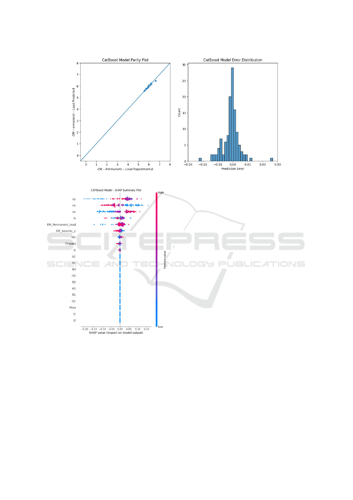
Figure 6: CATBoost Model Parity Plot and Error Distribution.

Figure 7: SHAP Values Summary Plot for CATBoost

Model.

5 DISCUSSION

Understanding the vulnerability of this system makes

it possible to plan targeted interventions, with the aim

of reducing or managing speciﬁc criticalities through

a prioritised programme of action, thus improving the

resilience and overall efﬁciency of the built fabric

against natural disasters. This system allows a vulner-

ability class to be assigned to each building through

a simpliﬁed analysis and quick consultation of pre-

deﬁned schemes. The adoption of this classiﬁcation

allows a quantitative assessment of structural perfor-

mance and is becoming a reference for future regula-

tions. The proposed work aims to deﬁne a protocol

for disaster mitigation and prevention through a nu-

merical approach based on an analytical analysis of

structural capacity curves. The main innovation of the

approach lies in the analysis method adopted, which

is based on a discontinuous ﬁnite element algorithm

that has already been extensively validated on various

case studies. This method provides direct and gener-

alisable results based on the structural morphology of

buildings. The canonical methods, which are based

on a direct mechanical analysis of the seismic capac-

ity of individual or aggregated buildings, while reli-

able, require a high level of knowledge of the struc-

tures and a high computational cost, making them im-

practical for urban-scale assessments. However, re-

cent developments in seismic risk and vulnerability

classiﬁcation methodologies have made it possible to

adopt a more rapid approach that allows direct esti-

mation of building damage following seismic events

and identiﬁcation of the most appropriate mitigation

measures. In this project, mechanical analysis mod-

els are integrated with data obtained from monitoring,

allowing quantitative and qualitative information use-

ful for risk management to be obtained. The approach

proposed for the Mitigation and Prevention Proto-

col overcomes the problem of the high computational

cost of the techniques currently used. The work pro-

poses to deﬁne the non-linear behaviour of a random

sample of buildings through a simpliﬁed pushover

procedure based on limit analysis. The integration of

machine learning techniques in the structural vulner-

AI4EIoT 2025 - Special Session on Artiﬁcial Intelligence for Emerging IoT Systems: Open Challenges and Novel Perspectives

478

ability assessment process and in the deﬁnition of the

Mitigation and Prevention Protocol introduces signiﬁ-

cant advantages in terms of efﬁciency, scalability and

accuracy of the analysis. The use of advanced ma-

chine learning algorithms makes it possible to pro-

cess large volumes of data from structural monitoring,

geospatial surveys and seismic event histories, allow-

ing correlations to be identiﬁed that are not immedi-

ately detectable with traditional methods. One of the

main beneﬁts of using machine learning is the abil-

ity to automate the classiﬁcation of the seismic vul-

nerability of buildings based on geometric, material

and construction characteristics, reducing the margin

of error associated with subjective assessments and

approximations of deterministic models. Deep learn-

ing algorithms, trained on extensive datasets, can im-

prove the prediction of damage scenarios through the

analysis of satellite images, LIDAR data and infor-

mation from sensors distributed in buildings. This

approach enables rapid assessments on a large scale,

facilitating the planning of targeted preventive inter-

ventions and optimising the allocation of resources.

Furthermore, the implementation of predictive mod-

els based on neural networks and advanced regression

techniques allows the estimation of structural capacity

curves to be reﬁned, improving the accuracy of sim-

pliﬁed pushover analysis. Through supervised learn-

ing, it is possible to develop early warning systems

capable of recognising premonitory signals of struc-

tural failure in real time, increasing the safety level of

buildings and urban infrastructure.

6 CONCLUSIONS

The use of machine learning (ML) models in the as-

sessment of the seismic vulnerability of buildings is

motivated by the need to develop efﬁcient predictive

tools, capable of processing large volumes of data

and adapting to variable conditions without the need

for simplifying assumptions imposed by traditional

methods. Compared to purely physical approaches,

such as ﬁnite element simulations, ML models allow

for a signiﬁcant reduction in calculation time, mak-

ing it possible to analyse a large number of struc-

tures in a short period of time. Furthermore, the abil-

ity of ML models to learn directly from experimen-

tal and numerical data allows for the identiﬁcation of

complex patterns that might not be immediately evi-

dent in models based exclusively on mechanical prin-

ciples. Compared to traditional statistical methods,

machine learning offers greater ﬂexibility and gener-

alisation capacity, reducing dependence on linear or

parametric assumptions. Integration with a physics-

based approach, based on the lower limit theorem of

limit analysis, also guarantees respect for the funda-

mental principles of structural mechanics, mitigating

the risk of obtaining predictions without a physical

basis. This combination of advantages makes the pro-

posed approach particularly suitable for tackling the

problem of assessing seismic vulnerability in a more

efﬁcient, robust and scalable way compared to alter-

native approaches. Finally, the combined use of ma-

chine learning with traditional numerical methodolo-

gies helps to reduce the processing time and compu-

tational cost of analyses, making assessments more

accessible even for large and complex urban contexts.

This synergy between artiﬁcial intelligence and struc-

tural engineering represents a decisive step towards

the creation of more resilient built environments ca-

pable of dynamically adapting to the stresses induced

by extreme events.

REFERENCES

Alber, M., Tepole, A. B., Cannon, W. R., De, S., Dura-

Bernal, S., Garikipati, K., Karniadakis, G., Lytton,

W. W., Perdikaris, P., Petzold, L., and Kuhl, E. (2019).

Integrating machine learning and multiscale model-

ing—perspectives, challenges, and opportunities in

the biological, biomedical, and behavioral sciences.

Barredo Arrieta, A., D

ıaz-Rodr

ıguez, N., Del Ser, J., Ben-

netot, A., Tabik, S., Barbado, A., Garcia, S., Gil-

Lopez, S., Molina, D., Benjamins, R., Chatila, R.,

and Herrera, F. (2020). Explainable artiﬁcial intelli-

gence (xai): Concepts, taxonomies, opportunities and

challenges toward responsible ai. Information Fusion,

58:82–115.

Breiman, L. (2001). Random forests. Machine Learning,

45(1):5 – 32.

Campanile, L., Di Bonito, L. P., Iacono, M., and Di Natale,

F. (2023). Prediction of chemical plants operating per-

formances: a machine learning approach. In Proceed-

ings - European Council for Modelling and Simula-

tion, ECMS, volume 2023-June, page 575 – 581.

Campanile, L., Di Bonito, L. P., Natale, F. D., and Iacono,

M. (2024). Ensemble models for predicting co con-

centrations: Application and explainability in envi-

ronmental monitoring in campania, italy. In Proceed-

ings - European Council for Modelling and Simula-

tion, ECMS, volume 38, page 558 – 564.

Chen, T. and Guestrin, C. (2016). Xgboost: A scalable tree

boosting system. In Proceedings of the ACM SIGKDD

International Conference on Knowledge Discovery

and Data Mining, volume 13-17-August-2016, page

785 – 794.

Ciaccio, F. D. and Troisi, S. (2021). Monitoring marine

environments with autonomous underwater vehicles:

A bibliometric analysis.

Damiano, E., Battipaglia, M., de Cristofaro, M., Ferlisi, S.,

Guida, D., Molitierno, E., Netti, N., Valiante, M., and

eXplainable Artiﬁcial Intelligence Framework for Structure’s Limit Load Extimation

479

Olivares, L. (2024). Innovative extenso-inclinometer

for slow-moving deep-seated landslide monitoring in

an early warning perspective. JOURNAL OF ROCK

MECHANICS AND GEOTECHNICAL ENGINEER-

ING.

de Cristofaro, M., Asadi, M. S., Chiaradonna, A., Dami-

ano, E., Netti, N., Olivares, L., and Orense, R. (2024).

Modeling the excess porewater pressure buildup in py-

roclastic soils subjected to cyclic loading. JOURNAL

OF GEOTECHNICAL AND GEOENVIRONMENTAL

ENGINEERING, 150.

Di Bonito, L. P., Campanile, L., Di Natale, F., Mastroianni,

M., and Iacono, M. (2024). explainable artiﬁcial intel-

ligence in process engineering: Promises, facts, and

current limitations. Applied System Innovation, 7(6).

Di Bonito, L. P., Campanile, L., Napolitano, E., Iacono,

M., Portolano, A., and Di Natale, F. (2023). Analy-

sis of a marine scrubber operation with a combined

analytical/ai-based method. Chemical Engineering

Research and Design, 195:613 – 623.

Dietterich, T. G. (2000). Ensemble methods in machine

learning. Lecture Notes in Computer Science (includ-

ing subseries Lecture Notes in Artiﬁcial Intelligence

and Lecture Notes in Bioinformatics), 1857 LNCS:1 –

15.

Domingos, P. (2012). A few useful things to know about

machine learning. Commun. ACM, 55(10):78–87.

eli5 Development Team (Accessed 2022). eli5 Documenta-

tion - Permutation Importance.

Gunning, D. and Aha, D. W. (2019). Darpa’s explainable ar-

tiﬁcial intelligence program. AI Magazine, 40(2):44–

58.

Guyon, I. and Elisseeff, A. (2003). An introduction to

variable and feature selection. J. Mach. Learn. Res.,

3(null):1157–1182.

Karpatne, A., Atluri, G., Faghmous, J. H., Steinbach, M.,

Banerjee, A., Ganguly, A., Shekhar, S., Samatova, N.,

and Kumar, V. (2017). Theory-guided data science:

A new paradigm for scientiﬁc discovery from data.

IEEE Transactions on Knowledge and Data Engineer-

ing, 29.

Ke, G., Meng, Q., Finley, T., Wang, T., Chen, W., Ma, W.,

Ye, Q., and Liu, T.-Y. (2017). Lightgbm: A highly ef-

ﬁcient gradient boosting decision tree. In Advances

in Neural Information Processing Systems, volume

2017-December, page 3147 – 3155.

Laub, J. A. (1999). Assessing the servant organization; de-

velopment of the organizational leadership assessment

(ola) model. dissertation abstracts international,. Pro-

cedia - Social and Behavioral Sciences, 1.

Lundberg, S. M. and Lee, S.-I. (2017). A uniﬁed approach

to interpreting model predictions. In Advances in Neu-

ral Information Processing Systems, volume 2017-

December, page 4766 – 4775.

Malami, S. I., Anwar, F. H., Abdulrahman, S., Haruna, S. I.,

Ali, S. I. A., and Abba, S. I. (2021). Implementation of

hybrid neuro-fuzzy and self-turning predictive model

for the prediction of concrete carbonation depth: A

soft computing technique. Results in Engineering, 10.

Mangalathu, S., Hwang, S.-H., and Jeon, J.-S. (2020). Ma-

chine learning-based failure mode identiﬁcation of re-

inforced concrete shear walls. Engineering Structures,

207:110257.

McGovern, A., Lagerquist, R., Gagne, D. J., Jergensen,

G. E., Elmore, K. L., Homeyer, C. R., and Smith,

T. (2019). Making the black box more transparent:

Understanding the physical implications of machine

learning. Bulletin of the American Meteorological So-

ciety, 100.

Momeny, M., Latif, A. M., Sarram, M. A., Sheikhpour, R.,

and Zhang, Y. D. (2021). A noise robust convolutional

neural network for image classiﬁcation. Results in En-

gineering, 10.

Pearson, K. (1895). Note on regression and inheritance in

the case of two parents. Proc. R. Soc. Lond., 58:240–

242.

Prokhorenkova, L., Gusev, G., Vorobev, A., Dorogush,

A. V., and Gulin, A. (2018). Catboost: Unbi-

ased boosting with categorical features. In Advances

in Neural Information Processing Systems, volume

2018-December, page 6638 – 6648.

Santhosh, A. J., Tura, A. D., Jiregna, I. T., Gemechu, W. F.,

Ashok, N., and Ponnusamy, M. (2021). Optimization

of cnc turning parameters using face centred ccd ap-

proach in rsm and ann-genetic algorithm for aisi 4340

alloy steel. Results in Engineering, 11.

Sharma, D. K., Jalil, N. A., Nassa, V. K., Vadyala, S. R.,

Senthamil, L. S., and Thangadurai, N. (2021). Deep

learning applications to classify cross-topic natural

language texts based on their argumentative form. In

Proceedings - 2nd International Conference on Smart

Electronics and Communication, ICOSEC 2021.

Vadyala, S. R., Betgeri, S. N., and Betgeri, N. P. (2022).

Physics-informed neural network method for solving

one-dimensional advection equation using pytorch.

Array, 13.

Vadyala, S. R., Betgeri, S. N., Sherer, E. A., and Amrit-

phale, A. (2021). Prediction of the number of covid-

19 conﬁrmed cases based on k-means-lstm. Array, 11.

Vadyala, S. R. and Sherer, E. A. (2021). Natural

language processing accurately categorizes indica-

tions, ﬁndings and pathology reports from multicenter

colonoscopy: Qualitative focus study (preprint). JMIR

Cancer.

Velliangiri, S., Alagumuthukrishnan, S., and Thankumar

joseph, S. I. (2019). A review of dimensionality re-

duction techniques for efﬁcient computation. Proce-

dia Computer Science, 165:104–111.

Zona, R., Ferla, P., and Minutolo, V. (2021). Limit anal-

ysis of conical and parabolic domes based on semi-

analytical solution. Journal of Building Engineering,

44.

Zona, R. and Minutolo, V. (2024). A dislocation-based ﬁ-

nite element method for plastic collapse assessment in

solid mechanics. Archive of Applied Mechanics.

AI4EIoT 2025 - Special Session on Artiﬁcial Intelligence for Emerging IoT Systems: Open Challenges and Novel Perspectives

480