Indexed Concatenation Notation: A Novel Way to Summarize Networks

and Other Complex Systems

Kenneth Caviness

, Colton Davis

1 b

, Derek Renck

1 c

, Charles Sarr

, Scot And erson

3 d

Heaven Robles

and Rhys Sh arpe

3 f

School of Engineering and Physics, Southern Adventist University, Taylor Circle, Collegedale, U.S.A.

Laurelbrook Academy, Campus Drive, Dayton, U.S.A.

School of Computing, Southern Adventist University, Taylor Circle, Collegedale, U.S.A.

Biology and Allied Health Department, Southern Adventist University, Taylor Circle, Collegedale, U.S.A.

Keywords:

Graph Identiﬁcation, Concatentation, Indexed Concatenation, Lossless Compression, Edge Difference Set

List.

Abstract:

The indexed concatenation notation presented in this paper extends the concept of concatenation in a way

similar to the extension of addition to the indexed sum, allowing compact representations of strings, lists,

matrices, etc., having internal repetitive or describable structure. In particular, it allows the edge difference

set list of any graphical network with a visible pattern to be summarized in an extremely compact and lossless

way. Examples highlight the information compression of the technique and showcase its ability to represent

complicated, inﬁnite patterns in closed form.

1 INTRODUCTIO N

Graph theory provides mathematicians and c omputer

scientists with many tools for the study of networks,

but none compactly id e ntify a large or inﬁnite net-

work. That situation has now changed: the Indexed

Concatenation Notation (ICN) allows any network

with a visible pattern to be “reduced” to form an ex-

tremely compact summary, which could then serve,

for example , as a “dictionar y entry” in a list of net-

works studied.

The notation deﬁned here owes much to the in-

dexed sum, product, union and n otations already

widely used in math e matics; it is a modern re incar-

nation of an idea N. G. de Bruijn jotted down in

1977 (de Bruijn, 1977). Although our direc t moti-

vation comes originally from graph theory, concate-

nation has deep roots in programming languages and

in computer science in gen eral. As far bac k as the

early 70s, the theory of concatenation included not

https://orcid.org/0009-0008-5240-6260

https://orcid.org/0000-0003-4348-7923

https://orcid.org/0009-0002-7564-2123

https://orcid.org/0009-0009-5053-555X

https://orcid.org/0009-0008-5434-7444

https://orcid.org/0009-0001-9671-3763

only strings, but lists as well (Campbell, 1971). Al-

most all programming languages include conca tena-

tion operators, but C can perform this opera tion in

at least ﬁve different ways, using either functio ns or

more primitive manipulations (WsCubeTech, 2025) .

Concatenation forms a fundamenta l operation in the

theory of computation, where it is essential in the un-

derstandin g of diff erent types of languag es from regu-

lar expressions to Turing machines (Sipser, 2012; Ma-

heshwari and Smid, 2024).

The prop osed extension of concatenation to allow

indexing strengthens the notation, which can then be

used with strings, lists, sequences, etc.

The ICN c a n be considered a new form of lossless

informa tion compression for strings, lists, sequences,

and networks.

2 MOTIVATION

In o ur work over several years, we have consistently

encountered networks having some obvious visual

pattern. One such example is shown in Figure 1.

Only a small part of the inﬁnite two-dimensional

network is shown, with the ﬁrst vertex of the graph in-

dicated by the small black arrow at the bottom right.

Caviness, K., Davis, C., Renck, D., Sarr, C., Anderson, S., Robles, H. and Sharpe, R.

Indexed Concatenation Notation: A Novel Way to Summarize Networks and Other Complex Systems.

DOI: 10.5220/0013514700003970

In Proceedings of the 15th International Conference on Simulation and Modeling Methodologies, Technologies and Applications (SIMULTECH 2025), pages 39-50

ISBN: 978-989-758-759-7; ISSN: 2184-2841

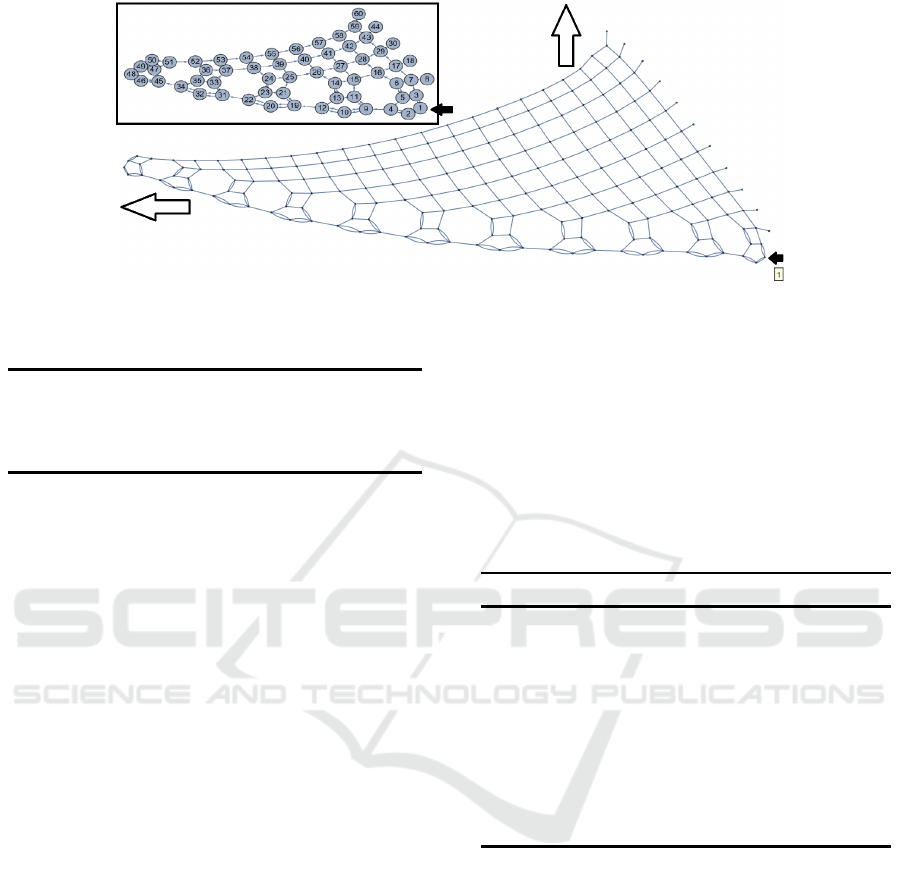
Figure 1: An inﬁnite two-dimensional network with a consistent internal pattern.

Table 1: The ﬁrst edges of the network shown in Figure 1.

1 → 2 1 → 2 1 → 3 1 → 3 2 → 4

2 → 4 3 → 5 3 → 7 4 → 5 4 → 9

5 → 6 5 → 6 6 → 7 6 → 16 7 → 8

7 → 17 9 → 10 9 → 10 9 → 11 9 → 11

The grap h grows without bound, extending indeﬁ-

nitely up and left. (See outlined arrows.) The small

inset shows the ﬁrst 60 vertices and edges between

them, with vertex numbers indicating the order in

which they were added to the graph as it was c on-

structed.

Although the layout is arbitra ry, the graph has

clear patterns along its growing edges and in its in-

terior. Visually, the lower edge of the graph is made

up of alternating pentagons and heptagons, with one

quadrilateral sitting on each pentagon. Each polygon

is made of single and double edges, always in the

same positions. The interior of the graph is single-

edged quadrilater a ls only, but the right-most one on

each row has a missing right side.

But such d escriptions are not deﬁnitive and might

apply equally well to many other networks. Similarly,

graph-theoretic prop e rties such as order and size (both

inﬁnite here), connectivity, vertex degrees, density,

girth, radius, diameter, height, etc., do not uniquely

identify a graph. It is frustrating to repeatedly come

across similar-seeming graphs that, o n closer inspec-

tion, turn out to be different. A graph is uniquely de-

ﬁned by its set of vertices and its set of edges, and

the only reliable identiﬁcation comes from consider-

ing those sets. We looked for ways to summarize this

data, without any loss of information. The ﬁrst few di-

rected edges of our example graph, sorte d by vertices

connected, are as shown in Table 1.

Any pattern visible to human eyes in the graph

above is hidden in this edge list, but the simple opera-

tion of ﬁrst grouping edges according to their starting

vertex and then taking the differences of starting and

ending vertex numbers for eac h edge sudd enly reveals

new vistas for the pa ttern seeker.

No information is lost in this process, since each

set, S

, completely speciﬁes the edges originating at

vertex i. The same information is in both the list of

edges (grouped by originating vertex) an d the edge

difference set list (EDSL ). Table 2 demo nstrates how

an EDSL is for med.

Table 2: Network edges and the corresponding EDS L.

Edges: EDSL:

{1 → 2, 1 → 2, 1 → 3,1 → 3} {1,1,2,2}

{2 → 4, 2 → 4} {2,2}

{3 → 5, 3 → 7} {2,4}

{4 → 5, 4 → 9} {1,5}

{5 → 6, 5 → 6} {1,1}

{6 → 7, 6 → 16} {1,10}

{7 → 8, 7 → 17} {1,10}

{} {}

{9 → 10, 9 → 10, 9 → 11,9 → 11} {1, 1,2,2 }

... ...

The EDSL of a n etwork having some intrinsic pat-

tern fre quently includes su bsequences of exact dupli-

cate sets, p roviding an obvious ﬁrst step toward re-

duction to a summary. When we see, for instance,

2 adjac e nt copies of {1,10}, 4 adjacen t copies of

{1,12}, 6 copies of {1,14}, 8 copie s of {1,16} , and so

on, we temporarily rep resent these duplicate subse-

quences by

[{1,10}],

[{1,12}],

[{1,14}],

[{1,16}], etc. (More on the notation shortly.)

Compressing those allows us to notice other similar

cases, and soon we have the ﬁrst reduction o f this

graph’s EDSL:

SIMULTECH 2025 - 15th International Conference on Simulation and Modeling Methodologies, Technologies and Applications

{{1,1, 2,2}, {2,2} , {2,4},{1, 5},{1,1},

[{1,10}],{} , {1,1, 2,2}, {2,2},{2,4},

{1,7},{1, 1},

[{1,12}],{} , {1,1, 2,2}, {2,2},

{2,4},{1, 9},{1,1},

[{1,14}],{} , {1,1, 2,2},

{2,2},{2, 4},{1,11}, {1,1},

[{1,16}],{} , ...

)

(1)

In this case no further reduction can be achieved

based on exact duplica te s of adjacent sets or exact

duplicates of subsequences, but each 7-element row

(subsequence) above has a common pattern, with only

3 numbers changing in each row. In the ﬁrst row,

these numbers are 5, 2, and 10; in the k

row, they

are 2k + 3, 2k, and 2k + 8. Befor e movin g on to the

details of the Indexed Concatenatio n Notation, glance

at the fully reduced form of this EDSL in all its glory.

(

∞

k=1

{1,1, 2,2},

j=1

[{2,2 j}],

{1,2k + 3}, {1,1},

i=1

[{1,2k + 8}], {}

#) (2)

Note the index variables, i, j and k, which have

been introduced. Just as one would expect b y anal-

ogy to an indexed summation, i, j and k take on the

initial value of 1 and are incremented until the spe ci-

ﬁed ﬁnal values are r eached: here, 2k, 2, and inﬁnity,

respectively. Assuming the pattern has been well es-

tablished and will continue inde ﬁnitely, we have suc-

ceeded in sum marizing the e ntire inﬁnite network’s

EDSL in two scant lines!

3 NOTATION AND PRECEDENTS

We deﬁne the operators both f or standar d and indexed

concatenation, explaining th e background of the cur-

rent indexed concatenation notation.

3.1 Binary (Inﬁx) Operator

There is no generally ac cepted bin ary operator for

concatenation. Different programming languages im-

plement different operators for strings, such as S

in C++, Java, Pascal, and Python; S

in PHP and

Perl; S

∗S

in Julia; S

||S

in SQL; S

in Ad a,

BASIC, an d .NET; S

∼ S

in D; S

//S

in Fortran;

ˆS

in F#; S

..S

in Lua; S

in Smalltalk and

APL; an d S

<> S

in Wolfram Mathematica. In our

opinion, each of these options has signiﬁcant draw-

backs, each having widely varying meanings in other

contexts. Nor would the situation be improved by

importing the function composition operator used in

mathematics: f

◦ f

Several langu ages, including Haskell, Zig, and E r-

lang use two consecutive plus signs (++) for concate-

nation, and in the case of H a skell, the shifted over-

strike (Unicode 1 0746, hex 29FA): ++. This symbol

overcomes many of the drawbacks of the others. We

propose to use it as the b inary or inﬁx version of co n-

catenation. For example, we write

{1,2, 3}++{5,4,3}++{7}= {1,2, 3,5,4 , 3,7} (3)

3.2 Indexed Operator

Consider o ther familiar notations, such a s sum, prod-

uct, and union, both simple (binary, two-argument)

and indexed oper ators:

∑

i=1

= a

+ a

(4)

∏

i=1

= a

·a

= a

(5)

[

i=1

= S

∪S

(6)

Some examples with numbers:

∑

i=1

i = 1 + 2 + 3 + 4 = 10 (7)

∏

i=1

i = 1 ·2 ·3 = (1)(2)(3) = 6 (8)

[

i=1



i,i



= {1, 1}∪{2,4}∪{3,9}∪{4,16}

= {1, 2,3,4, 9,16}

(9)

Each indexed operator is deﬁned as an extension

of the corresponding binary operator : + →

∑

, · →

∏

∪ →

. The sum and product use different symbols

for the two, while the indexed un ion of sets reuses the

binary operator symbol for the indexed case, as does

the intersection.

Having a choice of prec e dents to follow, we opt

for the following for indexed concatenation :

i=1

= S

++S

(10)

Indexed Concatenation Notation: A Novel Way to Summarize Networks and Other Complex Systems

We settled on the euro symbol, which exists

widely, but no t in this context, so no misunderstand-

ing should occur. Visually, it resembles a “C” for

“Concatenate”, and also resembles our choice for the

inﬁx concatenation operator, ++, selected from the

Haskell computer language.

We begin by closely following the indexed union,

deﬁning the indexed con catenation in terms of the

simple operator. Crucially, unlike indexed union, con-

catenation doe s not eliminate du plicates nor sort the

resulting list. For example,

i=1

{i,i

} = {1, 1}++{2,4}++{3,9}

++{4,16}= {1,1, 2,4,3, 9,4, 16}

(11)

Similar work has been attempted previously.

Nicolaas Govert “Dick” de Bruijn, a Dutch math-

ematician noted for his co ntributions to analysis,

number theory, com binatorics and logic, published a

memorandum describing a notation for both simple

and indexed concatenation (de Bruijn, 1977). While

we have based our ICN on the more familiar sum-

mation notation, de Bruijn’s approach is slightly less

intuitive. He uses a three-sided box over each item

to be concatenated , forming what he terms comb no-

tation. His deﬁnition s are solidly rooted in set theory

and include a recursive deﬁnition f or the indexed con-

catenation oper a tor. But their time had, apparently,

not yet come. “This one’s for you, Dick!”

4 DEFINITIONS

We deﬁne the concatenation operator as a pplying to

strings, sequen c es, lists (shown here as sets, but with

no presumed sorting or removal of duplicates), and

any other similar objects (Table 3). Notice that the

concatenation of two strings results in a string, that

of two lists gives a list, etc. In all ca ses this can b e

thought of as retaining th e outer delimiters (those be-

fore a

and after b

) while the inner delimiters, those

adjacent to the concatenation symbol (” ++ “, }++ {,

or ] ++ [), disappear with it. The use of curly braces

{} for lists aligns well with common usage for sets

in mathematics, where sequences are often shown

without delimiters, and occasionally with parenthe-

ses (Rehmann, 2020). The squar e brackets [] used

above for sequences is another nod to the Haskell lan-

guage, but we treat this as a vanishing delimiter (see

below).

Indexed c oncatenatio n (of any n objects S

of the

same type) is now deﬁned as a generalization of the

binary operator:

i=1

= S

++S

++... S

(12)

Of course, any index may be used, or if not essen-

tial for deﬁning the p rocess, it can be omitted. If the

initial value is omitted, a desired default (generally 1

or 0) should be speciﬁed. We saw examples of this in

the Motivation section.

5 SIMPLE EXAMPLES

We provide mu ltiple examples of the capabilities of

indexed concatenation when a pplied to lists, matr ic es,

and other datatypes. In each case indexed conca te na-

tions shows pro mising potential to concisely summ a -

rize repeated patterns.

5.1 Strings

Concatenation of strings works exactly as expected:

“ABC” = “ABC” ++“ABC” ++“ABC”

= “ABCABCABC”

(13)

Overloading the “+” operator to advance the char-

acter a certain number of steps in a given alphabet

(such as adding an int to a char in C-like languages),

allows this nested example:

i=0

j=0

(“A” + i + j) = “ABC” ++ “BCD”

++“CDE” ++“DEF” = “ABCBCDCDEDEF”

(14)

5.2 Integers and Digits

The notation might even extend to concaten a ting the

digits of numbers, when the argument is neither a list

nor a sequence, but an integer: the concatenation of

integers should be an integer.

i=1

= 1 ++4 ++9 ++16 ++25 = 1491625 (15)

That would be in contrast to using [], indicating a

sequence to be summarized:

i=1

] = [1] ++[4] ++ [9] ++[16] ++[25]

= [1,4, 9,16, 25]

(16)

SIMULTECH 2025 - 15th International Conference on Simulation and Modeling Methodologies, Technologies and Applications

Table 3: Operation of inﬁx concatenation on various datatypes.

Strings: “a

... a

” ++ “b

... b

” = “a

... a

...b

”

Lists: {a

,... ,a

} ++ {b

,... ,b

} = {a

,... ,a

,... ,b

}

Sequences: [a

,... ,a

] ++ [b

,... ,b

] = [a

,... ,a

,... ,b

]

Table 4: Examples of using indexed concatenation with digits.

Fraction Decimal Overline Notation Indexed Concatenation

0.333 ... 0.

3 0.

∞

0.142857142857 . . . 0.

142857 0.

∞

(142857)

200

111

1.801801801 1.

801 1.

∞

(801)

0.010010001 .. . 0.

∞

i=1



j=1



Table 4 provid e s several examples of compress-

ing digits with indexed concatenatio n. We note here

that the com mon overline notation looks m uch sim-

pler, and probably should be re tained except in cases

such as the last example, which is an irrational num-

ber.

5.3 Lists and Sequences

We now turn to indexed conc atenation of lists and se-

quences. Some examples:

i=1



i,i



= {1, 1}++{2, 4}++{3,9}

= {1, 1,2,4, 3,9}

(17)

i=1

{i,10 −i} = {1, 9}++{2,8}++{3, 7}

++{4,6}++{ 5,5} = {1,9, 2,8,3 , 7,4, 6,5,5 }

(18)

Again, the concatenation of lists is a list, without

adding nested levels of the list structure. Of course,

to make a list with sublists, we can nest the lists that

serve as input to the concatenation operator. A con-

catenation of lists with one level of sublists is a list

with one level of sublists:

i=1



i,i



= {{1, 1}}++{ {2,4}}

++{{3,9}}= {{1,1}, {2,4},{3, 9}}

(19)

With sequences, the only difference is that all se-

quence delimiters that remain after the concatena -

tion will vanish if inside another structure, so subse-

quences expand back out without add ing additional

levels of ne stin g. (Outer sequence delimiters remain,

so the following is a sequ e nce, not a list.)

i=1

j=1

[ ji] =

i=1

[i,2i,3i] = [1,2, 3]

++[2,4,6] ++[3 , 6,9] = [1, 2,3,2 , 4,6, 3,6,9 ]

(20)

But invoking the disapp earance of our seq uence-

delimiter when inside some other object, one c an con-

catenate subsequences in an outer list:

(

j=1

[ ji]

)

= {[1, 2,3,2, 4,6, 3,6,9 ]}

= {1, 2,3,2, 4,6, 3,6,9 }

(21)

These can be nested to any level desired. So we

have two ways to represent a list of integers having an

internal pattern. For example,

{1,1, 1,1, 1,2,2, 2,2, 1,1,1, 1,1, 2,2,2 , 2,1,

1,1, 1,1,2, 2,2, 2}→

(

[1],

[2],

[1],

[2],

[1],

[2]

)

→

(

[1],

[2]

(22)

Indexed Concatenation Notation: A Novel Way to Summarize Networks and Other Complex Systems

{1,1, 1,1, 1,2,2, 2,2, 1,1,1, 1,1, 2,2,2 , 2,1,

1,1, 1,1,2, 2,2, 2}→ {1, 1,1,1,1}++{2,2,2,2}

{1,1, 1,1, 1}++{2,2, 2,2}++{1,1,1, 1,1}

++{2,2,2,2 } →

{1}++

{2}

{1}++

{2}++

{1}++

{2}

→

{1}++

{2}

(23)

The above examples have primarily involved in-

creasing values, increasing numb er of values, or both.

However, because any formula based on the concate-

nation indices can be used, th is notation can also rep-

resent sequences involving descending numbers of el-

ements and descending values.

i=1



10−i



= {512,256,128, 64,32,16,8, 4, 2,1}

(24)

n=0

(

3−n

i=0

{3 −i −n}

)

= {{3, 2,1, 0},{2 , 1,0}, {1,0},{0}}

(25)

We can even produce Pascal’s Triangle, grouped

by rows, to any d e sired row. (Again, replacing th e

inner, {}, b y th e disappearing subsequence delim iters,

[], would produce a single list.)

n=0

(

k=0



k!(n −k)!



)

= {{1},{1, 1},{1,2,1},{1, 3, 3,1},

{1,4, 6,4, 1},{1, 5,10, 10,5, 1}}

(26)

5.4 Matrices

A generalized matrix (a

i j

), with 1 ≤i ≤ m, 1 ≤ j ≤n,

can be written in IC notation as a conc atenated list of

concatenate d lists:







··· a







i=1

(

j=1



i j



)

(27)

If the matrix has some additiona l structure, that

could also be shown explicitly in the IC f orm. For

example, in the matrix mechan ic s representation of

quantum p hysics, th e annihilation opera tor ˆa, which

lowers the quantum state |ni to |n −1i for a on e -

dimensional harmonic oscillator, is given in the en-

ergy eigenba sis by an inﬁnite matrix whose pattern

that can be explained in words: “All diagonal ele-

ments are zero. T he entries

√

n appear in the ﬁrst

subdiagonal above the diagonal. All other elements

are 0.” Yes, that is clear. But how much b etter to give

a mathematically precise deﬁnition in IC nota tion!







√

1 0 0 0 0 0 . ..

0 0

√

2 0 0 0 0 ...

0 0 0

√

3 0 0 0 ...

0 0 0 0

√

4 0 0 ...

0 0 0 0 0

√

5 0 ...

0 0 0 0 0 0

√

6 ...

0 0 0 0 0 0 0 ...







∞

k=1

((

[0],

√

∞

[0]

))

(28)

Very co ncise. Similarly, the inﬁnite matrix r e pre-

sentations of the creation ope rator ( ˆa

†

), the position

( ¯x), and mo mentum ( ˆp) operators, can all be written

in nested IC form .

6 CANTOR’S ENUMERATION OF

ALL FRACTIONS & THE

FAILURE OF SET-BUILDER

NOTATION

Finally, let’s consid er an example that will resonate

with math ematicians: the IC notation construc tion

of the ﬁrst enumeration of the rationals, published

in (Cantor, 1874). Georg Cantor, the father of trans-

ﬁnite mathematics, published his proof of the count-

ability of th e rationals in 1874, over 150 years ago.

One might presume that in the inter vening time some-

one would have come up with a concise, ma themati-

cally precise way to de scribe the process. Sadly, that

SIMULTECH 2025 - 15th International Conference on Simulation and Modeling Methodologies, Technologies and Applications

1/1

1/2

2/1

1/3

3/1

1/4

4/1

1/5

5/1

⋮

⋯

5/2 ⋯

5/3 ⋯

5/4 ⋯

5/5 ⋯

⋮ ⋮ ⋮ ⋮ ⋱

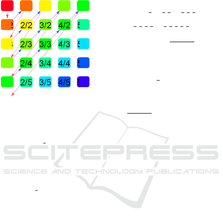
Figure 2: A traversal producing Cantor’s enumeration of

fractions.

expectation would be incorrect. Wor ds to describe

Cantor’s method are easy:

1. Imagine an inﬁnite tab le in which th e ﬁrst element

of the ﬁrst row is

, and then moving one column

to the right always incre ases the numera tor by 1,

while m oving one row down increases the denom-

inator by 1.

2. Following any (inﬁnite) row or column would

mean never getting to the next one; instead, we

traverse the array one (ﬁn ite) dia gonal at a time,

starting from the upper left corner. Note that for

all elements

on a given diagonal, n + d is a

constant, and in fact, o n diagonal number diag,

n + d = diag + 1.

Cantor actually used a “snake-like” traversal,

winding back-and-for th on alternate diagonals, but for

our purposes a “trace and retrace” pattern is prefer-

able.

Figure 2 ﬁrst appeared in (Caviness, 2011), and

the code to generate it was upd ated in (Nachbar,

2023).

The following IC constructs the diagonals in the

order Cantor visits them, but traverses each diago-

nal from left-to-right (by increasing numerator), as

shown by the small blue arrows, bef ore advancing to

the next diagonal (longer red arrows). We do this by

two nested IC objects, the outer specifying the diag-

onal diag, the inner giving the n

element on the di-

agonal. If the nested list structure is not desired, the

inner set of curly braces could be replaced by the dis-

appearin g square brackets, generating sequences that

are simply spliced into a single list.





















...



→

∞

diag=1

(

diag

n=1



1 + diag −n



)

(29)

This enumeration cannot be easily produced by

conventional mathematical notation, such as using

set-builder notation. For example,





p,q ∈Z



(30)

produces all fractions, but loses Cantor’s diagonal or-

dering.



diag −n + 1



diag ∈ Z

,n ∈{1, ..., diag}



(31)

again produces all fr actions, but assumes the user will

not sort the resulting list (i.e., non-standard trea tment

for sets), and has no in te rest in grouping entries by di-

agonal. The Indexed Concatenation form practically

writes itself, while set-builder notation requires sig-

niﬁcant mathematical gymnastics to produce the same

result.

7 A MULTIPLY-NESTED

EXAMPLE

One of the authors (Davis) created many inﬁnite net-

works having some visual symmetry and patterned

structure, identiﬁed vertices and edges for the begin-

ning of each graph (again following some clear, re-

peating pattern), con structed its EDSL and then re-

duced it. One interesting case consists of nested,

growing, interconnected pentagons, as shown in Fig-

ure 3.

The answer foun d, which completely deﬁnes this

structure out to the 8th penta gon, was this intere sting

triply nested structure.

(

n=1

{1,5n + 4,5n + 5},

k=1

i=1

[{1}], {1,k + 5n + 5}

n−1

j=1

[{1}], {}

(32)

Indexed Concatenation Notation: A Novel Way to Summarize Networks and Other Complex Systems

Figure 3: A multidimensional network with a triply nested

concatenation.

Expanding the outer IC levels shows an fascinat-

ing feature of the I C notation . Although by con-

struction all graph edges connect lower numbered ver-

tices to higher numbered ones, so the EDSL contains

only positive numbers, a 0 appeared in the ﬁnal IC

for n = 1, but only as the ending value for the in-

dex:

j=1

[{1}]. Further examples showed that a 0

or even a negative ending valu e is perf ectly legal for

an indexed concatenation: That subsequence is sim-

ply omitted from th e fully expanded list. Sim ilarly,

i=1

[{1}] only expands o ut to a single copy of {1}.

(

{1,9, 10},

i=1

[{1}], {1,11 },

i=1

[{1}], {1,12 },

i=1

[{1}], {1,13 },

i=1

[{1}], {1,14 },

j=1

[{1}], {},

{1,14,15} ,

i=1

[{1}], {1,16 },

i=1

[{1}], {1,17 },

i=1

[{1}], {1,18 },

i=1

[{1}], {1,19 },

j=1

[{1}], {},

{1,19,20} ,

i=1

[{1}], {1,21 },

i=1

[{1}], {1,22 },

i=1

[{1}], {1,23 },

i=1

[{1}], {1,24 },

j=1

[{1}], {},.. .

)

(33)

Clearly, once a pattern is d e te cted, it is worth try-

ing to extend it backwards in th e list: it may apply

even where not initially noticed. For reference, the

fully expanded EDSL begins in this way:

{{1, 9,10},{1},{1,11},{1},{1,12},{1},{1,13},

{1}, {1,14},{},{1,1 4,15}, {1},{1},{1,16},

{1}, {1}, {1,17},{1}, {1},{1,18},{1},{ 1},

{1,19},{1},{},{1,1 9,20}, {1},{1},{1},{1,21},

{1}, {1}, {1}, {1,22}, {1},{1},{1},{1,23},

{1}, {1}, {1}, {1,24}, {1},{1}, {},{1,24,25},

{1}, {1}, {1}, {1}, {1, 26},{1}, {1},{1},{1},

{1,27},{1},{1}, {1}, {1},{1, 28},{1},{1},

{1}, {1}, {1,29},{1}, {1},{1}, {},{1,29,30},. ..}

(34)

8 A SELECTION OF NETWORKS

Here is a small co llec tion of different networks we

have successfully compressed, each sh own together

with its c ompressed e dge difference set list (EDSL)

in indexed concatenation form (IC). Many of these in-

clude nested concatenatio ns. All of the networks can

be extend ed by in creasing the end value of the ind ex

variable in the outer indexed concatenation. Replac-

ing the end value by ∞ results in an inﬁnite network,

without adding any complexity to the IC form shown.

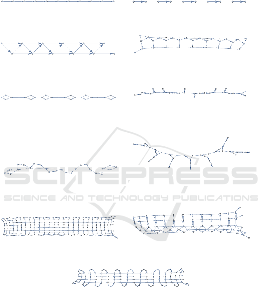
Figures 4 and 5 showcase the examples selected,

together with their concatenated EDSLs. Figure 4

consists of examples of networks that c a n extend in-

deﬁnitely in one dimension , whether or not a close

view appears one- or two-dimensional. (Cases that

are locally three-dimensional have also been found.)

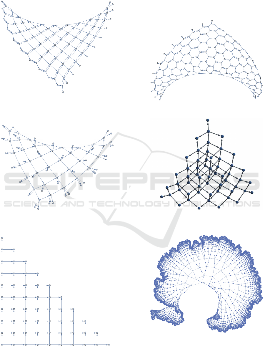
Figure 5 shows several higher-dimensional networks

along with their EDSLs. Most of these visually ap-

pear to be two-dimensional (expanding in two direc-

tions), and all include at least two levels of indexed

concatenation, one nested inside the other, although

such nesting does not guarantee two-dimensionality,

as can be seen from Figure 4.

One example (Figure 5d) is clearly three-

dimensional (expanding in three directions as the

outer index increases), an d is su mmarized by a three-

level nesting of indexed co ncatenation s. Yet others

we have investigated are too dense to “ﬁt” in three di-

mensions. Figure 5f provides an example of this last

type, which we refer to as growing “exponentially.”

At this point we have no clea r connection between IC

nesting and the “growth dimensionality” of the grap h

represented.

In each of these cases, a complex geometric pat-

tern is captured mathematically by indexed concate-

nation.

SIMULTECH 2025 - 15th International Conference on Simulation and Modeling Methodologies, Technologies and Applications

1 2 3 4 5 6 7 8 9 10 11

(a)



[{1}]



1 2 3 4 5 6 7 8 9 10

(b)



[{1},{}]



(c)



[{1,2}]



(d)



[{2,3},{3},{1,2}]



(e)





k=1

[{2k −1, 2k}],

[{1,2},

[{}]



(f)



[{2,2,2},{1,3,3},{2},{1,1,3},

{2},{1,1,1},{3}]}

(g)



[{2,3},{1, 2},{}]



(h)





{1,6,8}, {},



[2]





[3]



,{}



(i)



n=0



k=1

[{1,18 −2k}],

k=8

[{1,1}]



(j)





[{1,7,8}],

[{1,1,7}],{7},{},{}



(k)



n=0



k=1

[{1,12 −2k}],

k=5

[{1,1}]



Figure 4: A selection of networks and their concatenated EDSLs.

Indexed Concatenation Notation: A Novel Way to Summarize Networks and Other Complex Systems

(a)



i=1

[{1,1,1},{1,1,i + 1},

i−1

[{1,1,i + 2}], {i + 2,i + 3}



(b)



k=1



{2k −1, 2k + 1},

[{1,1},{1, 2k}]



(c)



k=1



k−1

[{},{1,1, 2,2k}],

{},{2k,2(k + 1)}]}

(d)



n=1



i=1





z =

n(n + 1),

z + i,z + i + 1}]]]}

(e)



k=1



[{k,k + 1}]



(f)

k=1



−1,2

+ 1





+ 1



,{1},

−1

j=1



1, j + 2

−1, j + 2



Figure 5: A selection of higher-dimensional networks and their EDSLs.

SIMULTECH 2025 - 15th International Conference on Simulation and Modeling Methodologies, Technologies and Applications

Figure 6: A two-dimensional network with multiple possi-

ble summarizations.

One network may have multiple possible summa-

rizations, as is demonstrated in Figure 6. This net-

work’s EDSL could be conca tenated as either

(

n=1

[{1,2, 3},{3n + 1, 3n + 2},{1,2},

{3n −1,3n + 1 },

n−1

[{1,2}],{3n,3n + 1}

{3n + 2,3n + 3 },{1,2, 3},{3n + 3, 3n + 4}, {1, 2},

{3n + 1,3n + 3 },

n−1

[{1,2}],{3n + 2,

3n + 3}],

{1,2},{1, 3n + 6}, {3n + 2,3n + 3}



(35)

or, alternatively, as

(

n=1

m=0

[{1,2, 3},{2m + 3n + 1,2m + 3n + 2},

{1,2},{2m + 3n −1,2m + 3n + 1},

n−1

[{1,2}],{2m + 3n,2m + 3n + 1}

[{1,2},{1, 3n + 6}], {3n + 2,3n + 3}



(36)

9 CONCLUSIONS

Throu ghout the history of mathematics and science,

good notation has contributed to incr e ased under-

standing, greater insights, and more rapid an d suc-

cessful ad vancement in the ﬁeld un der study. Ex-

amples include the decimal system (replacing previ-

ous use of Roman numerals a nd dependence o n frac-

tions), Leib nitz’ representation of the d e rivative of y

with respect to x as

, vector nota tion to conveniently

describe relationships in three-dimensional space, the

4-vector notation in Special Relativity to include the

time coordinate, and the summation convention used

in tensor calcu lus a nd General Relativity. G ood nota-

tion facilitates good work.

The Indexed Concatenation Nota tion, following

the lead of other indexed operators, allows compact

representations of strings, lists, sequences, integer

lists, matr ices, and other similar expressions, exam-

ples of which we have consid ered above. It ca pital-

izes on repetitions, p eriodicities and other patterns to

compress information into a reduced form. It may

be hoped that such notation summarizing internal pat-

terns may not only serve as a new mean s of informa-

tion compression, but also contribute to simpler and

more insightful use of the data.

10 PROSPECTS

Where do we go from here?

1. Fine- tune automated manipulation of IC notation.

Our code to partially or completely exp and out

Indexed Concatenation lists and sequences works

for any ﬁnite nestin g level. However, we have en-

countere d two main shortcomings:

(a) The reverse direction is harder; our algorithm

currently identiﬁes and reduces 70% o f the

sample ca ses a ttempted.

(b) Treatment of strings and integers has not yet

been implemented in either direction.

2. Publish a f ollow-up paper showcasing the algo-

rithm itself once the co de is further reﬁned.

3. Construct and/or ﬁnd other interesting graphs to

reduce.

4. Construct an algo rithm to generate an IC sum-

mary of the complete list o f the edges of a graph

from its EDSL (edge differences set list).

5. What e lse it might be used for?

(a) Musical scores of various music genres?

(b) Summarizing D NA seque nces?

Our research team is actively pursuing these op-

tions, in particular the a pplication of the IC notation

to music and bioinformatics and the reﬁnme nt of a

network su mmarization algorithm.

Indexed Concatenation Notation: A Novel Way to Summarize Networks and Other Complex Systems

ACKNOWLEDG EM EN TS

The authors acknowledge the generous su pport of the

Academic Research Comm ittee of Southern Adven-

tist University for funding this projec t and relate d

work which led to it.

REFERENCES

Campbell, J. (1971). Comparative survey of programming

languages. COMPUTING AS A LANGUAGE, pages

391–484.

Cantor, G. (1874).

Uber eine Eigenschaft des Inbegriffes

aller reellen algebraischen Zahlen. Journal f¨ur die

reine und angewandte Mathematik, 77:258–262.

Caviness, K. (2011). Indexing strings and rulesets. The

Mathematica Journal, 13.

de Bruijn, N. G. (1977). Notation for concatenation. Tech-

nical report, Technische Hogeschool Eindhoven.

Maheshwari, U. and Smid, M. (2024). Introduction to The-

ory of Computation. School of Computer Science,

Carleton University.

Nachbar, R. (2023). Reply t o changed meth-

ods for displaying graphs (networks).

https://community.wolfram.com/groups/-

/m/t/2862755?p

p auth=iQ7ZaUTu.

Rehmann, U. (2020). Sequence. https:

//encyclopediaofmath.org/in-dex.php?title=

Sequence&oldid=48671.

Sipser, M. (2012). Introduction to the Theory of Computa-

tion. Cengage Learning, 3rd edition.

WsCubeTech (2025). C program to concatenate two strings

(5 ways). https://www.wscubetech.com/resources/c-

programming/programs/concatenate-two-strings.

SIMULTECH 2025 - 15th International Conference on Simulation and Modeling Methodologies, Technologies and Applications