Machine Learning-Driven Framework for Identifying Parameter-Driven

Anomalies in Multiphysics Simulations

Zohreh Moradinia, Hans Vandierendonck and Adrian Murphy

Queen’s University Belfast, Belfast, U.K.

Keywords:

Multiphysics Simulations, Anomaly Detection, Machine Learning.

Abstract:

This paper addresses the critical challenges associated with error management in multiphysics simulations,

particularly regarding the sensitivity of these systems to parameter selection, which can lead to convergence

failures and anomalies in simulation outputs. We propose a comprehensive analytical framework that sys-

tematically identiﬁes the relationships between simulation parameters and governing equations, enabling the

analysis of resulting anomalies. The framework classiﬁes these anomalies, providing insights that inform

the selection of appropriate unsupervised machine-learning algorithms for effective anomaly detection. To

demonstrate the applicability of this approach, we apply the framework to a heat conjugate transfer (HCT)

problem, integrating the heat transfer and Navier-Stokes equations. By thoroughly investigating parameter-

driven anomalies, our framework enhances the reliability, convergence, and ﬁdelity of multiphysics simula-

tions, ultimately contributing to the robustness and accuracy of simulation outcomes.

1 INTRODUCTION

Multiphysics simulations are integral to a broad range

of scientiﬁc and engineering applications, provid-

ing detailed insights into complex systems that in-

volve interactions between multiple physical phe-

nomena. Traditional modelling approaches, includ-

ing numerical methods, analytical techniques, and

equivalent circuit models, are widely employed in

this ﬁeld. Numerical methods such as the Finite

Element Method (FEM) and Finite Volume Method

(FVM) are renowned for their accuracy and robust-

ness. However, their reliance on signiﬁcant computa-

tional power, memory, and time resources poses con-

siderable challenges, especially when simulating in-

tricate or large-scale systems (Rinaldi, 2001; Peter

H. Aaen and Balanis, 2006). In contrast, analyti-

cal methods are computationally efﬁcient and precise

but are typically restricted to simple geometries, lim-

iting their applicability to more complex structures

(Zhang, 2021). Similarly, equivalent circuit methods

simplify computational complexity but are inefﬁcient

for novel devices requiring iterative adjustment (Jun-

quan Chen and Xu, 2012).

The use of multiphysics simulations inherently in-

volves managing various sources of error. Errors in

these simulations can stem from modelling assump-

tions, numerical discretization, and ﬁnite-precision

arithmetic, and they can signiﬁcantly affect the ac-

curacy and reliability of the results (Oberkampf and

Trucano, 2002). Addressing these errors is critical,

particularly in high-consequence applications where

even small inaccuracies can have substantial impacts.

Modelling errors arise from incomplete representa-

tions of the physical system, round-off errors result

from limited numerical precision in computational

arithmetic, and discretization and truncation errors are

introduced during the discretization process of con-

tinuous equations (Heng Xiao and Roy, 2016; Tyson,

2018). These error sources necessitate careful miti-

gation strategies, such as grid reﬁnement, model cal-

ibration, and higher-order discretization schemes, to

improve simulation accuracy.

Despite the critical importance of minimizing er-

rors, maximizing precision in all aspects of a simu-

lation is often resource-intensive. Researchers fre-

quently adopt a conservative approach, prioritizing

maximum precision in parameter selection to ensure

accuracy and result convergence. However, this prac-

tice often leads to prolonged computational times,

even when high precision is not necessary for ev-

ery stage of the simulation. The challenge of bal-

ancing accuracy with computational efﬁciency has

been a persistent issue in the ﬁeld, as researchers

must often make trade-offs between simulation pre-

cision and performance (Committee, 1998; Christo-

278

Moradinia, Z., Vandierendonck, H. and Mur phy, A.

Machine Learning-Driven Framework for Identifying Parameter-Driven Anomalies in Multiphysics Simulations.

DOI: 10.5220/0013514200003970

In Proceedings of the 15th International Conference on Simulation and Modeling Methodologies, Technologies and Applications (SIMULTECH 2025), pages 278-286

ISBN: 978-989-758-759-7; ISSN: 2184-2841

pher J. Roy and Oberkampf, 2003; Christopher J. Roy

and McWherter-Payne, 2003; He and Ding, 2001).

This balance becomes even more complex when con-

sidering the uncertainty in input parameters, bound-

ary conditions, and material properties, which can ex-

acerbate the inherent uncertainty in multiphysics sim-

ulations.

Previous studies have proposed several ap-

proaches to address these challenges, including un-

certainty quantiﬁcation (UQ) methods and precision

control techniques. UQ is essential for assessing

how variability in model inputs inﬂuences simula-

tion outputs, but traditional UQ techniques such as

reduced-order modelling, polynomial chaos expan-

sions, and Monte Carlo sampling are computation-

ally expensive and often necessitate simplifying the

model (R. A. Adams and Schmid, 2012; Ghanem

and Spanos, 1991; Oakley, 2004). While these meth-

ods reduce the dimensionality or complexity of the

problem, they may inadvertently limit the scope of

the simulation or compromise its accuracy. More-

over, precision management strategies, such as adjust-

ing arithmetic precision or discretization step sizes,

have been explored to mitigate computational cost,

but their effectiveness is constrained by the conﬂict-

ing demands of accuracy and performance (Harvey

and Verseghy, 2016; V. Chandola and Kumar, 2009).

To address these limitations, this paper intro-

duces a novel approach leveraging machine learning

(ML)-based anomaly detection techniques for mul-

tiphysics simulations. the proposed technique iden-

tiﬁes anomalies—instances where simulation results

deviate from expected outcomes—without altering

the complexity of the simulation. This approach al-

lows for the monitoring of simulation performance

and the detection of critical points where errors accu-

mulate or accuracy is compromised, effectively serv-

ing as an early warning system for simulation fail-

ures. The key contribution of this paper is a machine

learning-based anomaly detection framework that en-

hances the accuracy and reliability of multiphysics

simulations while reducing computational costs. This

approach enables practitioners to make informed de-

cisions regarding precision levels and parameter se-

lection, thereby optimizing simulation performance

without sacriﬁcing accuracy. The proposed method

enables the exploration of a broader range of simu-

lation conﬁgurations while optimizing both precision

and computational efﬁciency.

In this study, we apply the proposed anomaly de-

tection technique to a heat conjugate transfer (HCT)

problem, using heat transfer and Navier-Stokes equa-

tions to illustrate its effectiveness in identifying sim-

ulation anomalies. This method provides a more ef-

ﬁcient and computationally feasible alternative to tra-

ditional error management strategies in multiphysics

simulations. Moreover, the approach facilitates a

deeper understanding of the trade-off between simu-

lation precision and performance, enabling the selec-

tive adjustment of parameters based on speciﬁc sim-

ulation needs to avoid the common practice of uni-

formly applying maximum precision and unnecessar-

ily resource-intensive.

2 METHOD

In this study, we present a framework for detecting

anomalies in multiphysics simulation results by an-

alyzing the relationship between effective parame-

ters and the governing physical equations. Our ap-

proach integrates multiphysics simulations with ML

anomaly detection algorithms. Speciﬁcally, we apply

this method to the conjugate heat transfer problem,

focusing on ﬂow over a heated plate. Open-source

solvers and coupling tools are utilized to conduct the

simulations. The methodology consists of three key

steps. First, we assess the inﬂuence of various pa-

rameters—including physical, material, and simula-

tion parameters—on the simulation outcomes. Un-

derstanding how these parameters affect the results is

crucial for identifying potential anomalies. Second,

we investigate the relationship between these parame-

ters and the governing equations to determine whether

improper parameter settings could adversely impact

the equations and, consequently, the simulation re-

sults. This analysis enables us to quantify the extent

to which incorrect parameter values contribute to de-

viations from expected outcomes. Finally, based on

the insights gained from the parameter-equation rela-

tionship, we select an appropriate ML anomaly de-

tection algorithm. A key requirement for the algo-

rithm is that it should not rely on predeﬁned labeled

data, as anomalies in simulation results can manifest

in diverse ways. Therefore, we employ unsupervised

learning algorithms, which do not require prior train-

ing on labeled datasets and making it ideal for rare

and unknown anomalies. Additionally, unsupervised

methods can identify previously unseen anomalies by

learning normal system behavior and effectively scale

to the large datasets typical of multiphysics problems.

Many unsupervised algorithms are also computation-

ally efﬁcient, making them suitable for real-time or it-

erative simulations.However, selecting the most suit-

able unsupervised algorithm depends on the speciﬁc

multiphysics problem, as it is inﬂuenced by both the

governing equations and the associated parameters.

To verify the model, we compare its outcomes when

Machine Learning-Driven Framework for Identifying Parameter-Driven Anomalies in Multiphysics Simulations

279

applied to simulation results obtained under different

conﬁgurations. Speciﬁcally, we examine cases where

the value of one of the effective parameters differs

from the default conﬁguration settings and compare

these results with the ground truth obtained from the

default simulation setup. This comparison allows us

to assess the model’s ability to detect anomalies and

validate its accuracy in identifying deviations caused

by parameter variations. Ultimately, this framework

enables the development of a model that assists in

conﬁguring simulations appropriately for a given ap-

plication. It provides valuable insights into simula-

tion results, facilitating the identiﬁcation of anomalies

speciﬁc to the problem. Moreover, it aids in optimiz-

ing the balance between computational speed and ac-

curacy based on application requirements, enhancing

the overall efﬁciency and reliability of multiphysics

simulations.

3 CASE STUDY

Conjugate heat transfer (CHT)(M. Vynnycky and

Pop, 1998) is a critical phenomenon that involves the

transfer of heat between ﬂuids and solid boundaries,

where heat passes from one ﬂuid to the solid bound-

ary and then transfers from the solid to the other ﬂuid.

This process is particularly important in engineering

applications such as heat exchanger design and cool-

ing systems for electronic components.

In this study, we focus on a two-dimensional CHT

problem involving a rectangular, thermally conduct-

ing slab with laminar, incompressible ﬂuid ﬂow over

it. This scenario presents a classic CHT challenge,

where the steady heat transfer dynamics must be ac-

curately captured to ensure reliable simulation results.

The forced ﬂow occupies the region −∞ ≤ x ≤ ∞, y >

0, with uniform velocity U

and temperature T , while

the conducting slab occupies the region −a ≤ y ≤ 0,

−

≤ x ≤

. A schematic of this setup is illustrated in

Figure 1. To accurately model this problem, two gov-

erning equations are used: the Navier-Stokes equa-

tion for ﬂuid motion and the heat transfer equation for

Figure 1: Physical model and coordinate system of ﬂow

over heated plate.

temperature distribution. The Navier-Stokes equation

governs the motion of the ﬂuid and can be written as:

= −∇p + µ∇

v + f , (1)

Where ρ is the ﬂuid density, v is the velocity, p is the

pressure, and µ is the ﬂuid viscosity. This equation ac-

counts for both convection and diffusion in the ﬂuid’s

motion. The heat transfer equation, which governs the

temperature distribution in the system, is expressed

as:

ρc

= ∇ · (k∇T ) +Q, (2)

where ρ is the density, c

is the speciﬁc heat capacity

at constant pressure,

is the substantial (material)

derivative of temperature, k is the thermal conductiv-

ity, and Q is the volumetric heat generation rate.

To simulate ﬂuid ﬂow and heat transfer, we uti-

lize OpenFOAM (H. Jasak, 2007)software, employ-

ing the laplacianFoam solver for steady-state heat

conduction in solid slabs and the buoyantPimpleFoam

solver for buoyancy-driven ﬂuid ﬂow and transient

simulations using the PIMPLE algorithm. Accurate

coupling of solvers for ﬂuid and solid domains in

CHT simulations is addressed with PreCICE soft-

ware(H. J. Ungartz, 2016), which ensures consistent

heat ﬂux and temperature transfer between regions,

enhances accuracy at the solid-ﬂuid interface, and im-

proves performance through iterative methods, effec-

tive solver communication, and data mapping for non-

matching grids. This multiphysics problem analyzes

heat ﬂux and temperature exchange to determine how

key parameters—including time step, convergence

limitation, CP, Reynolds number, and Prandtl num-

ber—impact the heat and Navier-Stokes equations,

identifying simulation discontinuities, as outlined in

Table 1.

4 STUDING EFFECTIVE

PARAMETERS

In managing the precision and computational efﬁ-

ciency of simulations, there is a tendency to avoid

conﬁguring all parameters at the highest precision due

to the signiﬁcant increase in computational cost and

execution time. However, when parameters are not set

to these high-precision values, anomalies may emerge

in the simulation results. Figures 2 illustrate the com-

plex relationship between time steps and heat capac-

ity in relation to the output parameters of the simula-

tion. Each data point on these graphs corresponds to a

unique simulation conﬁguration. In this study, errors

are deﬁned as the mean difference between the simu-

lation outputs for a given parameter conﬁguration and

SIMULTECH 2025 - 15th International Conference on Simulation and Modeling Methodologies, Technologies and Applications

280

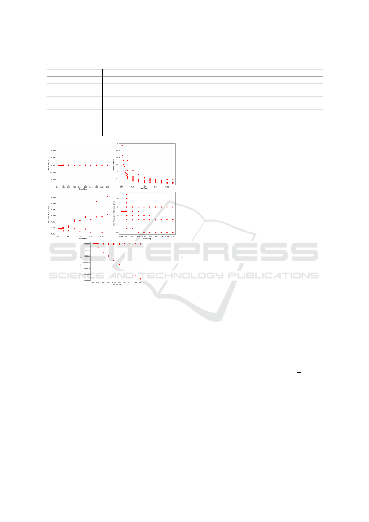
Table 1: Deﬁnition of studied Parameters in HCT problem.

Parameter Deﬁnition

Time Step The discrete intervals for simulation progression, affecting accuracy and stability.

Convergence Limita-

tion

A threshold that indicates when the iterative solution has achieved acceptable accuracy based on differ-

ences between iterations.

CP The heat required to change a unit mass of a material by one degree Celsius, affecting its temperature

response and heat transfer.

Reynolds Number A dimensionless parameter that classiﬁes ﬂuid ﬂow as laminar or turbulent based on inertial versus

viscous forces.

Prandtl Number A dimensionless ratio that indicates the relative importance of momentum transfer to heat transfer in

ﬂuid ﬂows.

Figure 2: Time-steps versus selected outputs in ﬂow over

heated plate problem- average error of temperature and ﬂux,

ﬁnal residual, iteration numbers, and execution time

those obtained using the default conﬁguration. Figure

2 highlights the minimal error range observed for both

the average temperature and the ﬁnal residual values,

with negligible error in the ﬂux average across all time

steps. Notably, the uniformity in the number of iter-

ations across different time steps underscores the ro-

bustness of the results. Importantly, our ﬁndings in-

dicate that increasing the time step size results in a

nearly 50% reduction in execution time while main-

taining high simulation accuracy, with errors below

0.05% for the temperature output.

These results suggest that a wide range of parame-

ter conﬁgurations can be used without compromising

simulation precision, enabling faster simulations. The

insights gained from our ﬁndings help to elucidate the

complexities involved in multiphysics simulations, re-

vealing important relationships between critical pa-

rameters and their outcomes. The ﬂexibility to ad-

just parameter values, while it may slightly impact

accuracy, is crucial in optimizing simulations for efﬁ-

ciency.

5 ANALYSIS OF PARAMETER IN

HEAT TRANSFER AND

NAVIER-STOKES EQUATIONS

This section explores the inﬂuence of the Reynolds

number (Re), Prandtl number (Pr), CP, and numerical

modelling parameters such as time step and conver-

gence limitations on the solutions of the heat transfer

and Navier-stokes equations. We aim to understand

their potential to create or smooth out discontinuities

in the temperature ﬁeld and heat ﬂux.

5.0.1 Non-Dimensional Form of Heat Transfer

Equations

To understand the effects of the Re, Pr, and c

, we

non-dimensionalize the heat transfer equation. below

are dimensionless variables:

∗

T − T

∞

∆T

, u

∗

, x

∗

, t

∗

, (3)

where: U is a characteristic velocity, L is a charac-

teristic length, T

∞

is the reference temperature, ∆T is

the temperature difference. Substituting these into the

heat conduction equation, we ﬁrst need to express all

terms in terms of the dimensionless variables. Start

with the substantial derivative term. Substitute the di-

mensionless variables:

T = T

∞

+ T

∗

∆T, u = Uu

∗

, x = Lx

∗

,t =

∗

. (4)

This is the non-dimensional form of the heat conduc-

tion equation:

∂T

∂t

+ u · ∇T =

Re · Pr

∇

T +

ρc

U∆T

. (5)

5.0.2 Non-Dimensionalization of the

Navier-Stokes Equations

The non-dimensionalization process can be applied to

the Navier-Stokes equations to better understand how

Machine Learning-Driven Framework for Identifying Parameter-Driven Anomalies in Multiphysics Simulations

281

various parameters inﬂuence heat ﬂux.

∗

, P

∗

ρU

, x

∗

, t

∗

(6)

Where U is a characteristic velocity, L is a character-

istic length, P represents pressure, ρ is density. After

substituting and rearranging, the Navier-Stokes equa-

tions in their dimensionless form can be expressed as:

∂u

∗

∂t

∗

+ u

∗

· ∇

∗

= −∇

∗

∇

∗2

∗

+ F

∗

(7)

Here, F

∗

represents body forces expressed in non-

dimensional form.

5.1 Effects of Physical Parameters in

Heat Transfer and Navier-Stokes

Equations

The analysis of temperature and heat ﬂux can be

signiﬁcantly affected by physical parameters. Un-

derstanding these parameters is crucial for detecting

anomalies caused by not incorrect values of these pa-

rameters

5.1.1 Reynolds Number (Re)

Re is a dimensionless quantity that characterizes the

ﬂow regime of a ﬂuid, representing the ratio of inertial

forces to viscous forces. It is deﬁned as:

Re =

ρU L

(8)

where ρ is the ﬂuid density, U is the characteristic

velocity, L is the characteristic length, and µ is the

dynamic viscosity. In high Reynolds number scenar-

ios, the convective term u·∇T dominates over the dif-

fusive term

Re·Pr

∇

T , leading to stronger convective

heat transfer and sharper temperature gradients, espe-

cially near walls (thermal boundary layers). Turbu-

lence enhances mixing, smoothing temperature dis-

continuities in the bulk ﬂow while maintaining rapid

temperature changes near boundaries.

At low Reynolds numbers, viscous and thermal

diffusion become more signiﬁcant, with the term

Re·Pr

∇

T being larger. This enhances thermal diffu-

sion, smoothing temperature gradients and resulting

in a more orderly ﬂow with smoother temperature dis-

tributions.

In regions with high shear, such as near solid

boundaries, substantial velocity gradients can arise,

leading to abrupt changes in the velocity ﬁeld, creat-

ing potential discontinuities and turbulence.

5.1.2 Prandtl Number (Pr)

Pr is another essential dimensionless quantity that re-

lates the momentum diffusivity (kinematic viscosity)

to thermal diffusivity, deﬁned as:

Pr =

(9)

where ν is the kinematic viscosity and α is the thermal

diffusivity. In high Pr scenarios, momentum diffu-

sivity is signiﬁcantly greater than thermal diffusivity.

The term

Re·Pr

becomes small, making the thermal

diffusion term ∇

T less inﬂuential. Consequently,

the temperature gradient near surfaces can be steep,

leading to pronounced thermal gradients and poten-

tial discontinuities. The Navier-Stokes equations can

be approximated as:

∂u

∂t

+ u · ∇u = −

∇P +

∇

u (10)

The reduced thermal diffusion in high Pr conditions

can result in prolonged high temperature gradients,

which can induce potential discontinuities near solid

boundaries or within ﬂows exhibiting signiﬁcant ther-

mal stratiﬁcation. Conversely, when Pr is low, ther-

mal diffusivity becomes more effective, leading to a

thicker thermal boundary layer and smoother temper-

ature distributions. In this regime, the thermal dif-

fusion term ∇

T is more signiﬁcant, enhancing the

conduction effect and reducing the likelihood of tem-

perature discontinuities.

5.1.3 Speciﬁc Heat Capacity (c

)

The speciﬁc heat capacity (c

) plays a pivotal role in

determining the thermal response of a ﬂuid, deﬁning

the amount of heat required to change the temperature

of a unit mass by one degree Celsius. A higher c

in-

dicates that the ﬂuid can absorb more heat before ex-

periencing signiﬁcant temperature changes, smooth-

ing out temperature gradients. This increased thermal

inertia also raises the thermal time constant:

τ =

ρc

(11)

Conversely, a low c

allows for a more rapid tem-

perature increase in response to heat inputs, which

can create sharper temperature gradients and increase

the likelihood of discontinuities, particularly in re-

gions with high heat ﬂux. Although c

does not ex-

plicitly appear in the Navier-Stokes equations, it in-

ﬂuences the coupled energy equation: This equation

shows that a higher c

increases the thermal inertia of

the ﬂuid, resulting in smoother temperature variations

and reducing discontinuities in both velocity and tem-

perature ﬁelds, as the ﬂuid takes longer to respond to

thermal changes.

SIMULTECH 2025 - 15th International Conference on Simulation and Modeling Methodologies, Technologies and Applications

282

5.2 Numerical Modeling Considerations

5.2.1 Time Step (∆t)

The time step ∆t in numerical simulations affects both

stability and accuracy. A smaller ∆t improves the

resolution of temporal changes, capturing transient

phenomena and reducing numerical artifacts, lead-

ing to more accurate and stable solutions, though at

higher computational cost. The Courant-Friedrichs-

Lewy (CFL) condition, ∆t <

, ensures stability by

limiting ∆t based on grid size and velocity, preventing

instabilities and artiﬁcial discontinuities. Conversely,

a larger ∆t can cause numerical instability, leading to

oscillations, divergence, and errors in the temperature

ﬁeld. Violating the CFL condition with a large time

step can result in unphysical results and the propaga-

tion of numerical errors.

5.2.2 Convergence Limitation

Numerical convergence is vital for accurate solutions,

and issues can arise from inadequate meshing, im-

proper boundary conditions, or insufﬁcient iterations,

leading to errors or discontinuities in the temperature

ﬁeld. A ﬁne mesh resolves small-scale features, with

the mesh size ∆x satisfying ∆x <

for N grid points

per characteristic length L, while insufﬁcient mesh-

ing can cause aliasing and artiﬁcial discontinuities.

Proper boundary conditions are essential to avoid un-

physical solutions, and they must match the physical

problem and be applied consistently to prevent spuri-

ous gradients. Sufﬁcient iterations are also necessary

for solvers to converge accurately, and meeting con-

vergence criteria like residual norms ensures stable,

accurate solutions. Incomplete convergence leaves

unresolved gradients and potential discontinuities.

6 ANOMALY DETECTION FOR

HCT

Based on the equations governing the parameters

studied in Section 6, setting parameters beyond ac-

ceptable limits may cause the convective term u · ∇T

to dominate over the diffusive term

Re·Pr

∇

T . This

dominance leads to stronger convective heat transfer

and sharper temperature gradients. When the term

Re·Pr

becomes small, the thermal diffusion term ∇

loses inﬂuence, resulting in steep temperature gradi-

ents near surfaces, which can cause signiﬁcant ther-

mal gradients and potential discontinuities.

When parameter values exceed the recommended

range, the dominant terms in the governing equations

can lead to anomalies and discontinuities in the simu-

lation results.

To avoid surpassing acceptable error thresholds,

limitations, or introducing discontinuities in the sim-

ulation results, we incorporate an additional step of

anomaly detection.

Speciﬁcally, we evaluate the effectiveness of three

anomaly detection algorithms—One-Class SVM, Iso-

lation Forest, and LOF to identify anomalies in tem-

perature and heat ﬂux data generated from the simu-

lations. These algorithms provide an important layer

of analysis to detect deviations that could indicate

emerging errors or inconsistencies in the results, help-

ing to maintain the integrity of the simulations.

6.1 Local Outlier Factor

The LOF (M. M. Breunig and Sander, 2000) is an un-

supervised anomaly detection algorithm that identi-

ﬁes anomalies by assessing local density deviations

of data points relative to their neighbors. It is particu-

larly effective in datasets with heterogeneous density

distributions, where the density of data points varies

signiﬁcantly across different regions.

The algorithm ﬁrst computes the k-distance for

each data point, deﬁned as the distance to its k-th

nearest neighbor. The choice of k critically inﬂuences

the sensitivity to anomalies; smaller k captures ﬁne

anomalies, while larger k identiﬁes broader patterns.

LOF computes reachability distances, which are

deﬁned for points A and B as the maximum of the

actual distance between A and B and the k-distance

of point B. This calculation ensures local density is

accurately represented.

The LRD for each point is derived as the in-

verse of the average reachability distance to its k-

nearest neighbors, reﬂecting the density of surround-

ing points.

LOF scores are calculated as the average ratio of

the LRD of a point’s neighbors to its own LRD. A

score near 1 indicates a normal point, while a score

signiﬁcantly greater than 1 indicates an anomaly.

6.2 One-Class SVM

The One-Class SVM(K.-L. Li and Xu, 2003) is an

unsupervised machine learning algorithm speciﬁcally

designed for anomaly detection. It is utilized to iden-

tify data points that signiﬁcantly deviate from the nor-

mal data distribution. Unlike conventional SVMs,

which are primarily used for binary classiﬁcation,

the One-Class SVM is trained exclusively on normal

data. Its goal is to construct a decision boundary that

encloses the majority of the normal data points, al-

Machine Learning-Driven Framework for Identifying Parameter-Driven Anomalies in Multiphysics Simulations

283

lowing the detection of anomalies that lie outside this

boundary.

SVM operates by receiving a dataset consisting

solely of normal data points, along with a kernel

function that transforms the input data into a higher-

dimensional space. This transformation is key to

enhancing the algorithm’s ability to separate normal

data points from potential anomalies, as it enables

the construction of a hyperplane in this transformed

space.

Once the decision function is learned based on the

normal data, it is applied to classify new data points.

Points that lie outside the established decision bound-

ary are classiﬁed as anomalies, while those within

the boundary are considered normal. Each new data

point is assigned an anomaly score, where negative

values denote normal points, and positive values indi-

cate anomalies.

6.3 Isolation Forest

Isolation Forest(F. T. Liu and Zhou, 2008) is an

unsupervised machine learning algorithm designed

for anomaly detection by recursively partitioning the

data. The underlying principle of Isolation Forest is

that anomalies are ”few and different,” making them

more susceptible to isolation than normal data points.

By constructing random decision trees, the algorithm

isolates individual data points and measures the path

length from the root to the point as an indicator of nor-

mality: shorter paths suggest anomalies, while longer

paths correspond to normal points.

Isolation Forest receives a dataset consisting of N

data points, along with predeﬁned parameters such as

the maximum tree height h and the number of trees

T to be generated. It begins by constructing multi-

ple isolation trees, each of which recursively parti-

tions the data by selecting random features and ran-

dom split values within the feature’s range. The pro-

cess continues until each data point is isolated or the

maximum tree height is reached.

For each data point, the path length in each tree is

computed, representing the number of splits required

to isolate that point. By averaging the path lengths

across all trees, the algorithm assigns an anomaly

score to each point. Data points that are isolated

quickly (i.e., have shorter path lengths) are more

likely to be anomalies, while those requiring longer

path lengths are more likely to be normal.

In this study, we employed several algorithms

to detect discontinuities in heat transfer simulations

caused by numerical errors, parameter variations, or

physical phenomena. Both One-Class SVM and

Isolation Forest effectively manage high-dimensional

spaces, which is crucial for the complexity of heat

transfer simulations involving multiple interacting pa-

rameters. Additionally, the LOF excels in identifying

anomalies within datasets characterized by varying

local densities, a common occurrence in heat trans-

fer simulations where temperature and heat ﬂux can

differ signiﬁcantly across regions. Furthermore, Iso-

lation Forest is notably efﬁcient and capable of han-

dling large-scale simulations, making it well-suited

for real-time anomaly detection in extensive heat

transfer datasets. Overall, these unsupervised learn-

ing methods improve the detection of discontinuities,

enhancing the reliability and accuracy of multiphysics

simulations. Their capabilities in managing high-

dimensional data, accommodating local density varia-

tions, and processing large datasets render them valu-

able tools for anomaly detection in complex engineer-

ing problems.

7 RESULTS AND DISCUSSION

In this section, we sought to identify the most effec-

tive method for detecting discontinuities in the sim-

ulation results. Each algorithm was assessed based

on its ability to detect anomalies without generating

excessive false positives, particularly in the context

of subtle parameter variations. The simulation out-

puts using default parameters are presented in Fig-

ure 3. The temperature and ﬂux data exhibit smooth

and continuous behaviour in the plots, with no evi-

dence of discontinuities or abrupt changes in the base-

line truth data simulation. It is essential to identify

any discontinuities or sharp transitions that may arise

due to variations in the studied parameter values using

algorithmic detection methods. Anomalies in simu-

lation results associated with different conﬁgurations

have been identiﬁed based on these analyses.

Figure 3: Temperature and Heat ﬂux plots of ﬂow over a

heated plate simulation.

Figure 4 illustrates anomaly detection across

three algorithms and each subplot represents varia-

tions in parameters with temperature and heat ﬂux

data. The black line represents the baseline, while

anomalies are marked: blue squares for IF, green cir-

cles for SVM, and red crosses for LOF.

SIMULTECH 2025 - 15th International Conference on Simulation and Modeling Methodologies, Technologies and Applications

284

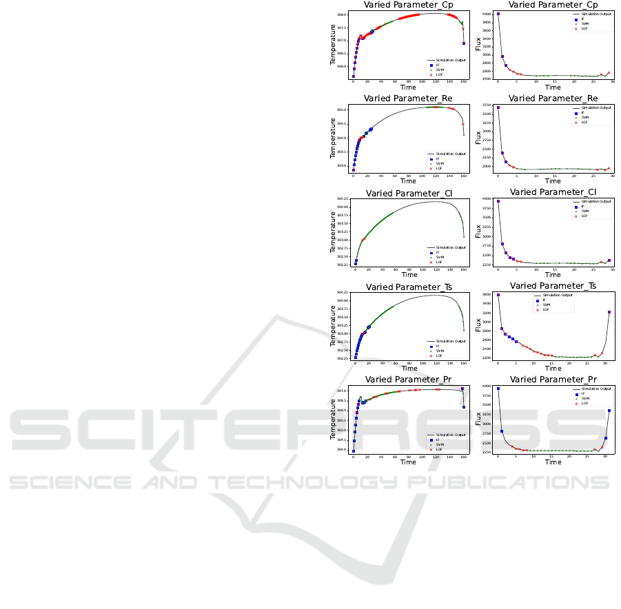
1. Anomaly Detection in Temperature Data: The

right column of plots shows temperature over time

for each varied parameter, generally following an ini-

tial rise before stabilizing, indicating thermal equili-

bration. This pattern helps evaluate each algorithm’s

ability to detect anomalies during both transient and

steady-state phases. The IF algorithm detects a few

anomalies, especially during the early rise phase, sug-

gesting it is more attuned to signiﬁcant outliers than

to smaller deviations. SVM detects more anoma-

lies overall, reﬂecting higher sensitivity to variations,

though this may increase false positives, especially

during a steady state. LOF, using local density, effec-

tively identiﬁes anomalies in the early, high-variance

phase, making it valuable for rapid-change regions,

though its detections decrease as the system stabi-

lizes.

2. Anomaly Detection in Heat Flux Data: The left

column shows heat ﬂux over time for each parameter.

Unlike temperature, heat ﬂux spikes initially, then de-

cays to a steady state, reﬂecting the system’s thermal

gradient settling into equilibrium.

IF detects a few anomalies, mainly during the ini-

tial spike, focusing on signiﬁcant deviations and over-

looking minor ﬂuctuations in the stable phase. SVM

detects anomalies consistently, including in stable pe-

riods, highlighting its sensitivity but with the potential

for false positives as ﬂux stabilizes. LOF captures a

high density of anomalies in the initial, rapid-change

phase but fewer as ﬂux reaches a steady state, show-

ing its strength in non-equilibrium conditions.

Parameter variations affect each algorithm

uniquely. Changes in Cp strongly impact temperature

and heat ﬂux, yielding high anomaly counts across all

algorithms. In contrast, Re primarily affects inertial

forces, resulting in fewer detections. Ts and Pr, which

directly inﬂuence thermal gradients, prompt higher

sensitivity: Ts variation causes rapid temperature and

ﬂux spikes, detected well by LOF and SVM, while

Pr changes create anomalies during the transition to a

steady state, effectively captured by IF and LOF.

The comparative analysis across various param-

eter changes highlights the critical balance between

sensitivity and speciﬁcity in anomaly detection al-

gorithms. One-Class SVM and Isolation Forest, de-

spite their capabilities, suffer from over-detection is-

sues that compromise their reliability, particularly

when variations are present. Conversely, LOF demon-

strated consistent accuracy and robustness in identi-

fying meaningful anomalies, suggesting it is the pre-

ferred method for ensuring the integrity of simulation

results in the presence of parameter variations.

Figure 4: Anomaly detection results of Isolation Forest, one

class SVM and LOF on Heat Flux and Temperature quan-

tity of ﬂow over a heated plate when selected parameters

changed.

8 CONCLUSION

The challenges associated with managing accuracy

and computational efﬁciency in multiphysics simu-

lations have long been a focus of research. The

necessity to balance precision and performance has

underscored the demand for innovative solutions.

This paper introduces a novel machine learning-based

anomaly detection framework that enhances the re-

liability of simulations by identifying critical points

where errors may arise. The key strength of our pro-

posed approach lies in its ability to optimize simula-

tion performance while maintaining accuracy, provid-

ing insights into the trade-off between precision and

computational cost. Our results demonstrate the ef-

fectiveness of this approach in heat transfer problems,

showcasing its versatility and potential applicability

across various scenarios. Importantly, this method-

ology simpliﬁes the error management process, sig-

Machine Learning-Driven Framework for Identifying Parameter-Driven Anomalies in Multiphysics Simulations

285

niﬁcantly reducing computational volume while en-

suring the integrity of the simulation outcomes. This

framework not only enhances the efﬁciency of multi-

physics simulations but also establishes a solid foun-

dation for conﬁdently determining optimal precision

requirements, marking a meaningful advancement in

the ﬁeld.

REFERENCES

Christopher J. Roy, M. A. M.-P. and Oberkampf, W. L.

(2003). Veriﬁcation and validation for laminar hyper-

sonic ﬂowﬁelds, part 1: Veriﬁcation. AIAA Journal,

41(10):1934–1943.

Christopher J. Roy, W. L. O. and McWherter-Payne, M. A.

(2003). Veriﬁcation and validation for laminar hyper-

sonic ﬂowﬁelds, part 2: Validation. AIAA Journal,

41(10):1944–1954.

Committee, C. F. D. (1998). Guide for the Veriﬁcation and

Validation of Computational Fluid Dynamics Simula-

tions (AIAA G-077-1998 (2002)). American Institute

of Aeronautics and Astronautics, Inc.

F. T. Liu, K. M. T. and Zhou, Z.-H. (2008). Isolation forest.

In Proceedings of the 2008 Eighth IEEE International

Conference on Data Mining, pages 413–422. IEEE.

Ghanem, R. and Spanos, P. (1991). Polynomial chaos in

stochastic ﬁnite elements. Journal of Applied Me-

chanics, 57(1):197–205.

H. J. Ungartz, F. Lindner, B. G.-e. a. (2016). precice—a

fully parallel library for multi-physics surface cou-

pling. Computers & Fluids, 141:250–258.

H. Jasak, A. Jemcov, Z. T. e. a. (2007). Openfoam: A c++

library for complex physics simulations. In Interna-

tional Workshop on Coupled Methods in Numerical

Dynamics, pages 1–20.

Harvey, R. and Verseghy, D. L. (2016). The reliability

of single precision computations in the simulation of

deep soil heat diffusion in a land surface model. Cli-

mate Dynamics, 46:3865–3882.

He, Y. and Ding, C. H. (2001). Using accurate arithmetics

to improve numerical reproducibility and stability in

parallel applications. The Journal of Supercomputing,

18:259–277.

Heng Xiao, J.-L. Wu, J.-X. W. R. S. and Roy, C. J. (2016).

Quantifying and reducing model-form uncertainties in

reynolds-averaged navier–stokes simulations: A data-

driven, physics-informed bayesian approach. Journal

of Computational Physics, 324:115–136.

Jun-quan Chen, Xing Chen, C.-J. L. K. H. and Xu, X.-B.

(2012). Analysis of temperature effect on pin diode

circuits by a multiphysics and circuit cosimulation

algorithm. IEEE Transactions on Electron Devices,

59(11):3069–3077.

K.-L. Li, H.-K. Huang, S.-F. T. and Xu, W. (2003). Improv-

ing one-class svm for anomaly detection. In Proceed-

ings of the 2003 International Conference on Machine

Learning and Cybernetics (IEEE Cat. No. 03EX693),

volume 5, pages 3077–3081. IEEE.

M. M. Breunig, H. P. Kriegel, R. T. N. and Sander, J. (2000).

Lof: Identifying density-based local outliers. ACM

SIGMOD Record, 29(2):93–104.

M. Vynnycky, S. Kimura, K. K. and Pop, I. (1998). Forced

convection heat transfer from a ﬂat plate: The conju-

gate problem. International Journal of Heat and Mass

Transfer, 41(1):45–59.

Oakley, J. E. (2004). Using latin hypercube sampling in un-

certainty analysis of complex models. In Proceedings

of the 2004 IEEE International Conference on Sys-

tems, Man and Cybernetics, volume 4, pages 3275–

3280.

Oberkampf, W. L. and Trucano, T. G. (2002). Veriﬁca-

tion and validation in computational ﬂuid dynamics.

Progress in Aerospace Sciences, 38(3):209–272.

Peter H. Aaen, J. A. P. and Balanis, C. A. (2006). Mod-

eling techniques suitable for cad-based design of in-

ternal matching networks of high-power rf/microwave

transistors. IEEE Transactions on Microwave Theory

and Techniques, 54(7):3052–3059.

R. A. Adams, D. J. I. and Schmid, C. T. (2012). Reduced

order modelling for simulations of nonlinear dynam-

ical systems. SIAM Journal on Scientiﬁc Computing,

34(3):A1273–A1296.

Rinaldi, N. (2001). On the modeling of the transient ther-

mal behavior of semiconductor devices. IEEE Trans-

actions on Electron Devices, 48(12):2796–2802.

Tyson, W. C. (2018). On numerical error estimation for the

ﬁnite-volume method with an application to computa-

tional ﬂuid dynamics. PhD thesis, Virginia Tech.

V. Chandola, A. B. and Kumar, V. (2009). Anomaly de-

tection: A survey. ACM Computing Surveys (CSUR),

41(3):1–58.

Zhang, Y. (2021). Improved numerical-analytical thermal

modeling method of the pcb with considering radia-

tion heat transfer and calculation of components’ tem-

perature. IEEE Access, 9:92925–92940.

SIMULTECH 2025 - 15th International Conference on Simulation and Modeling Methodologies, Technologies and Applications

286