Warm-Starting the VQE with Approximate Complex Amplitude

Encoding

Felix Truger

, Johanna Barzen

, Frank Leymann

and Julian Obst

Institute of Architecture of Application Systems, University of Stuttgart, Universit

atsstraße 38, Stuttgart, Germany

Keywords:

Variational Quantum Algorithm, Eigenvalues, Warm-Start, Classical Shadows.

Abstract:

The Variational Quantum Eigensolver (VQE) is a Variational Quantum Algorithm (VQA) to determine the

ground state of quantum-mechanical systems. As a VQA, it makes use of a classical computer to optimize

parameter values for its quantum circuit. However, each iteration of the VQE requires a multitude of measure-

ments, and the optimization is subject to obstructions, such as barren plateaus, local minima, and subsequently

slow convergence. We propose a warm-starting technique, that utilizes an approximation to generate beneﬁcial

initial parameter values for the VQE aiming to mitigate these effects. The warm-start is based on Approximate

Complex Amplitude Encoding, a VQA using ﬁdelity estimations from classical shadows to encode complex

amplitude vectors into quantum states. Such warm-starts open the path to fruitful combinations of classical

approximation algorithms and quantum algorithms. In particular, the evaluation of our approach shows that

the warm-started VQE reaches higher quality solutions earlier than the original VQE.

1 INTRODUCTION

Quantum computers are expected to excel in tasks

directly related to the properties of quantum me-

chanical systems, e.g., in quantum chemistry and

condensed matter physics (Feynman, 1982; Preskill,

2018; Tilly et al., 2022; Peruzzo et al., 2014). The

Variational Quantum Eigensolver (VQE) is a hy-

brid quantum-classical algorithm to obtain the ground

state energy of a given Hamiltonian operator describ-

ing such a system. As a Variational Quantum Al-

gorithm (VQA), the VQE is suited for current Noisy

Intermediate-Scale Quantum (NISQ) devices with

limitations in the width and depth of executable quan-

tum circuits (Preskill, 2018; Leymann and Barzen,

2020). Therefore, the VQE makes use of param-

eterized quantum circuits executed on NISQ hard-

ware and optimization algorithms executed on clas-

sical computers. This hybrid quantum-classical ap-

proach is deemed promising in the current era, where

quantum computers are still error-prone and limited in

number of qubits. Despite the bright prospects for the

VQE, several potential obstacles remain (Tilly et al.,

2022): To evaluate the energy of a system, each opti-

https://orcid.org/0000-0001-6587-6431

https://orcid.org/0000-0001-8397-7973

https://orcid.org/0000-0002-9123-259X

https://orcid.org/0000-0002-1898-2167

mization step of the VQE requires a multitude of mea-

surements depending on the composition of the given

Hamiltonian. Moreover, the optimization landscape

may be hard to navigate due to adverse effects such

as barren plateaus and local optima, and the algorithm

may exhibit insufﬁcient convergence properties.

Warm-starts are known for their capability to

mitigate some of these obstacles in quantum algo-

rithms (Truger et al., 2024). Warm-starting tech-

niques focus on the utilization of known or efﬁciently

generated results instead of starting an algorithm from

scratch, e.g., by making use of previous results or ef-

ﬁcient approximation algorithms. Several kinds of

warm-starting techniques affect quantum algorithms

in different ways. For example, there are two major

entry points for warm-starts of VQAs: Initial states

and initial variational parameter values. On the one

hand, such warm-starts can be realized through the

encoding of prior knowledge into the initial state of

a quantum circuit (cf. Egger et al., 2021; Tate et al.,

2023). Thereby, the initial state is biased towards fa-

vorable solutions, as opposed to neutral initial states

frequently assumed in conventional quantum algo-

rithms. On the other hand, warm-starts for VQAs can

be realized by providing viable initial values for the

parameters of the quantum circuit instead of a random

parameter initialization, e.g., by transferring optimal

parameter values from related problem instances or

Truger, F., Barzen, J., Leymann, F. and Obst, J.

Warm-Starting the VQE with Approximate Complex Amplitude Encoding.

DOI: 10.5220/0013513400004525

In Proceedings of the 1st International Conference on Quantum Software (IQSOFT 2025), pages 15-26

ISBN: 978-989-758-761-0

precomputing beneﬁcial parameter initializations, (cf.

Galda et al., 2021; Mitarai et al., 2022; Sack and Ser-

byn, 2021; Shaydulin et al., 2023).

Encoding approximate eigenvectors via amplitude

encoding yields a simple biased initial state to warm-

start the VQE. However, this warm-start is imprac-

tical due to the inefﬁciency of the encoding and

current hardware limitations. Moreover, it imposes

certain restrictions on the Ansatz of the VQE, as

we further elaborate in Section 4. In this work,

we utilize Approximate Complex Amplitude Encoding

(ACAE) (Mitsuda et al., 2024) to convert this idea into

a warm-start via parameter initialization, that is more

suitable for current hardware. By means of a ﬁdelity

estimation from so-called classical shadows (Huang

et al., 2020), the variational ACAE algorithm pro-

vides an efﬁcient approximate amplitude encoding of

complex vectors into a quantum state. We evaluate the

performance beneﬁts of the resulting warm-started

VQE (henceforth WS-VQE) over the standard VQE.

The underlying warm-starting technique employed in

WS-VQE can be used as a blueprint for other VQAs.

The remainder of this paper is organized as fol-

lows: In Section 2, we introduce the background and

fundamentals for this work. Section 3 discusses re-

lated work and Section 4 introduces WS-VQE, which

is evaluated and analyzed in Section 5. The results are

further discussed in Section 6 and the paper is con-

cluded with a summary and outlook in Section 7.

2 BACKGROUND AND

FUNDAMENTALS

We introduce VQE and ACAE in more detail to pro-

vide the background and fundamentals for WS-VQE.

2.1 Variational Quantum Eigensolver

The VQE follows the general construction of VQAs,

i.e., it is a hybrid quantum-classical algorithm based

on a parameterized quantum circuit, frequently re-

ferred to as Ansatz, and a classical optimizer (Peruzzo

et al., 2014; Cerezo et al., 2021). The Ansatz aims to

prepare a quantum state that represents a solution to

the problem instance at hand. The classical optimizer

iteratively adjusts the parameter values for the Ansatz,

which is in turn executed on a quantum device to as-

sess the current solution and navigate to an optimum.

Peruzzo et al. (2014) introduced the VQE to de-

termine eigenvalues of operators more efﬁciently than

possible with Quantum Phase Estimation. At its heart,

the VQE makes use of Quantum Expectation Estima-

tion (QEE), a subroutine that evaluates the expecta-

tion value of the given Hamiltonian for the state pre-

pared by the Ansatz. For the measurements on the

quantum computer, the Hamiltonian is decomposed

into a real-valued linear combination of tensor prod-

ucts of the identity I and the Pauli operators X, Y ,

and Z. The overall expectation value of the Hamilto-

nian H is computed as per Equation (1), i.e., as the

weighted sum of the expectation values of each Pauli

string P

in the linear combination, where x

are the

real-valued coefﬁcients of H’s Pauli decomposition.

⟨H⟩ =

∑

⟨P

⟩ (1)

Therefore, the state prepared by the Ansatz needs

to be measured multiple times for different measure-

ment bases as prescribed by the Pauli decomposition.

These measurements require the preparation of mea-

surement circuits with appropriate rotations to adjust

the measurement basis for each qubit. However, there

are various strategies of grouping Pauli strings that

can be measured jointly, which can reduce the num-

ber of measurement circuits signiﬁcantly (Tilly et al.,

2022). Nonetheless, the QEE subroutine typically re-

quires a multitude of measurement circuits to cover

all Pauli strings composing H. Each measurement on

a quantum computer typically needs to be repeated

multiple times to obtain results of a certain preci-

sion. These measurements are commonly referred

to as shots. Therefore, a hyperparameter N

shots

de-

termines the number of shots executed for measuring

each Pauli string. Thus, the total number of shots re-

quired for each call of the QEE subroutine amounts to

shots

× n

meas.circuits

, where n

meas.circuits

is the number

of measurement circuits, i.e., the number of groups of

jointly measurable Pauli strings.

The variational optimization of the VQE’s Ansatz

parameters aims to prepare a state that minimizes H’s

expectation value. Optimization typically starts from

a random initial parameterization or beneﬁcial val-

ues determined through speciﬁc methods (Tilly et al.,

2022). Thereby, the VQE eventually prepares an

approximate ground state of H with the lowest ex-

pectation. Potential applications include determining

electronic ground state energies and molecular poten-

tial energy surfaces in quantum chemistry (Li et al.,

2019), strongly correlated systems in condensed mat-

ter physics (Head-Marsden et al., 2021), protein fold-

ing for drug discovery (Mustafa et al., 2022; Barkout-

sos et al., 2021), material design (Barkoutsos et al.,

2021), and chemical engineering (Bernal et al., 2022).

The remainder of this work focuses on the underlying

mathematical problem tackled with the VQE, namely

to determine the lowest eigenvalue and corresponding

eigenvector of Hermitian matrices.

IQSOFT 2025 - 1st International Conference on Quantum Software

2.2 Approximate Complex Amplitude

Encoding

Amplitude encoding refers to encoding a vector

⃗

x ∈ C

with

⃗

x = (x

,. . . , x

n−1

) of unit length into the

amplitudes of a quantum state

⃗

⟩

, as shown in Equa-

tion (2) (Schuld and Petruccione, 2018).

⃗

⟩

n−1

∑

i=0

⟩

(2)

Its main advantage is that storing data of length n re-

quires only log n qubits. However, exact amplitude

encoding is infeasible because a circuit depth of at

least

is required for the preparation of an arbi-

trary state on n qubits (Schuld and Petruccione, 2018;

Shende et al., 2006). Approximate amplitude encod-

ing (Nakaji et al., 2022) suggests a VQA that approxi-

mately encodes vectors into the amplitudes of a quan-

tum state by training a shallow Ansatz. However, it

only supports the encoding of real-valued data.

Recently, Mitsuda et al. (2024) proposed Approxi-

mate Complex Amplitude Encoding (ACAE) based on

classical shadows (Huang et al., 2020). A classical

shadow is an approximate classical description of a

quantum state that is generated with few measure-

ments. It can be used to estimate different properties

of the captured quantum state. In the case of ACAE,

classical shadows are employed to estimate the ﬁ-

delity between a model state with the density operator

model

(θ) and a target state with the density operator

target

. Based on the estimated ﬁdelity, an Ansatz can

be variationally optimized to approximately encode

the target state described by ρ

target

. Classical shadows

are created by applying random unitary transforma-

tions to the state before measurements. For the ﬁ-

delity estimations in ACAE, the random unitaries are

taken from the n-qubit Clifford group. Results of mul-

tiple shots with different unitaries are averaged to ob-

tain an expectation value. The general idea is to clas-

sically undo these steps for each measurement result

. The averaging operation is viewed as a quantum

channel M , that is reverted by the inverse M

−1

. To

undo the random Clifford unitary U, the inverse trans-

formation U

†

is applied. The result

of undoing

these operations is called a snapshot:

= M

−1



†

⟩⟨



(3)

A classical shadow of the original state is a col-

lection of N

snaps

snapshots. From this approximate

classical description of the state, we can estimate cer-

tain properties. For instance, the expectation value of

an observable. Since the expectation value of an ob-

servable O in a state with the density operator ρ is

⟨O⟩ = Tr(Oρ), it is estimated by ⟨

O⟩ in Equation (4).

⟨

O⟩ =

snaps

∑

i=1

Tr(O

) (4)

Setting O = ρ

target

allows us to estimate the ﬁdelity

in ACAE. As shown in the supplementary material

provided by Huang et al. (2020), M

−1

boils down to

−1

(ρ) = (2

+ 1)ρ − I (5)

Thus, the ﬁdelity can be estimated by

f (θ):

f (θ) =

snaps

∑

i=1

Tr(ρ

target

)

snaps

∑

i=1

+ 1)⟨

target

†

⟩ − 1

(6)

Mitsuda et al. (2024) used ACAE to perform am-

plitude encoding of data for a quantum classiﬁer.

3 RELATED WORK

Tilly et al. (2022) provide a comprehensive review of

the VQE as well as methods and best practices related

to it, however, not explicitly focusing on warm-starts

for the VQE. Truger et al. (2024) conducted a map-

ping study for research on warm-starting techniques

in the quantum computing domain, including warm-

starts applicable to the VQE: Zhang et al. (2021) pro-

pose an adaptive construction of Ansatz circuits that

takes information obtained from a classical approx-

imation into account. Grimsley et al. (2023) pro-

pose dynamically growing the Ansatz during the ex-

ecution of the VQE and recycling previous parame-

terizations. Moreover, the VQE is compatible with

meta-learning, i.e., classical machine learning mod-

els trained to take over the task of the optimizer in

VQAs (Verdon et al., 2019; Wilson et al., 2021), and

plugging together multiple optimization steps that uti-

lize optimized parameters from one step to initialize

the next (Tao et al., 2023). Most relevant to our work,

various techniques for the parameter initialization of

the VQE have been proposed. Machine learning en-

ables generating circuits and viable initial parameter

values for each problem instance, that can be further

optimized (Dborin et al., 2022; Rudolph et al., 2023).

Exploiting the classically feasible simulation of Clif-

ford circuits can yield viable parameter initializations

for the VQE (Ravi et al., 2022; Mitarai et al., 2022).

Other approaches try to obtain viable parameter ini-

tializations for a parameterized Hamiltonian, thus tak-

ing advantage of the continuity of the problem to

obtain initializations for any parameterization of the

Warm-Starting the VQE with Approximate Complex Amplitude Encoding

ȁ ۧ

Ԧ𝑣

ȁ ۧ

VQE

Ansatz

𝑣

ACAE

Ansatz

ȁ ۧ

𝑣

ACAE

Ansatz

ȁ ۧ

VQE

Ansatz

𝜃

𝐶

VQE

Ansatz

ȁ ۧ

𝑣

VQE

Ansatz

ȁ ۧ

𝜃

𝐶

𝟏 𝟎 𝟑

𝟎 𝟎 𝟏

𝟑 𝟏 𝟐

ȁ ۧ

VQE

Ansatz

≈ Ԧ𝑣

𝑣 𝜃

𝟏 𝟎 𝟑

𝟎 𝟎 𝟏

𝟑 𝟏 𝟐

𝐶

a) Standard VQE b) WS-VQE with Biased Initial State

c) WS-VQE with Biased Initial State via ACAE

d) WS-VQE with Parameter Initialization via ACAE

≈ Ԧ𝑣

𝟏 𝟎 𝟑

𝟎 𝟎 𝟏

𝟑 𝟏 𝟐

𝟏 𝟎 𝟑

𝟎 𝟎 𝟏

𝟑 𝟏 𝟐

𝟏 𝟎 𝟑

𝟎 𝟎 𝟏

𝟑 𝟏 𝟐

𝟏 𝟎 𝟑

𝟎 𝟎 𝟏

𝟑 𝟏 𝟐

𝟏 𝟎 𝟑

𝟎 𝟎 𝟏

𝟑 𝟏 𝟐

𝟏 𝟎 𝟑

𝟎 𝟎 𝟏

𝟑 𝟏 𝟐

𝟏 𝟎 𝟑

𝟎 𝟎 𝟏

𝟑 𝟏 𝟐

Problem Instance

(Hermitian Matrix)

Approximate Solution

(Eigenvector)

ACAE/VQE

Parameters

Random Clifford

Measurements

OUR

APPROACH

ACAE Pre-Training

ACAE/VQE Pre-Training

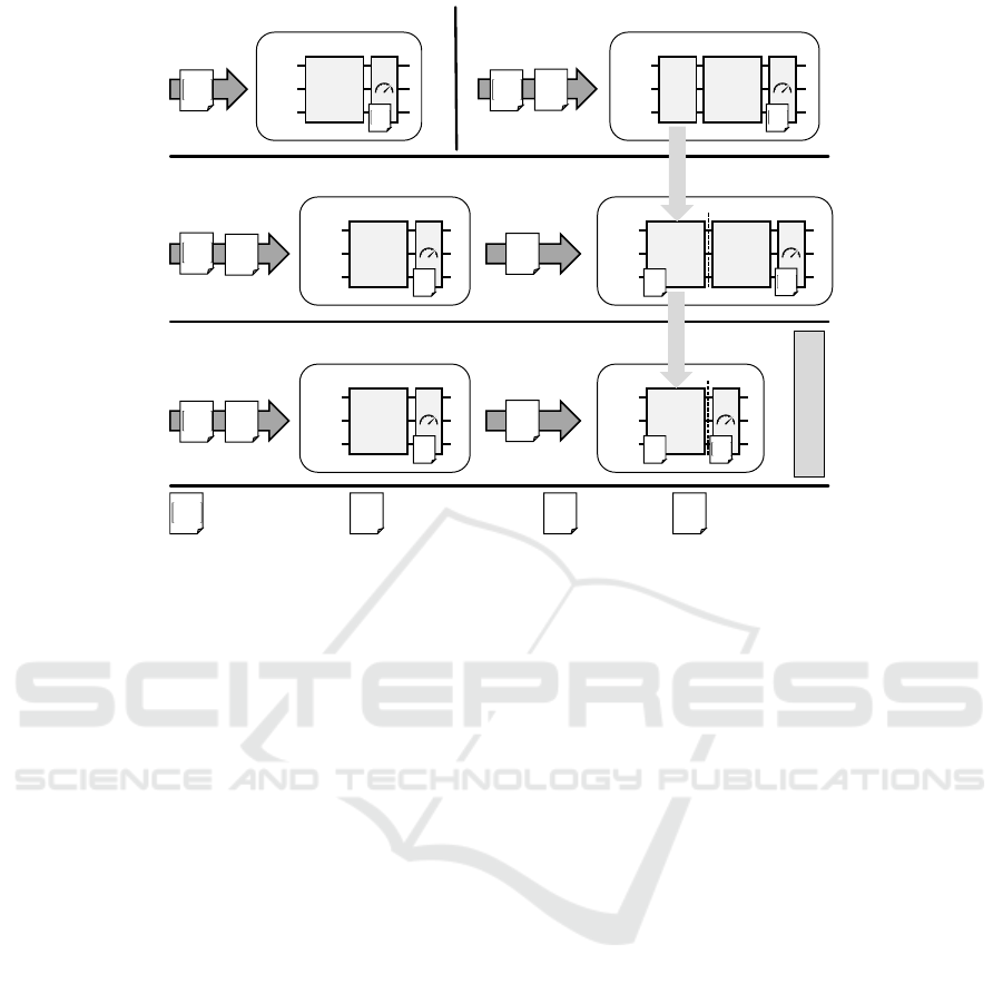
Figure 1: Shaping WS-VQE: a) The standard VQE without warm-start. b) A simple warm-start for the VQE using amplitude

encoding to prepend a biased initial state based on an approximate eigenvector ⃗v to the VQE Ansatz. c) A warm-start for the

VQE that prepends a pretrained ACAE Ansatz instead of amplitude encoding. d) Our approach, a warm-start for VQE based

on ACAE pretraining of the VQE Ansatz to approximately encode a given approximate eigenvector.

Hamiltonian (Cervera-Lierta et al., 2021; Harwood

et al., 2022). Similarly, the VQE has been shown to be

compatible with parameter transfers, where optimized

parameters from one instance are reused to initialize

the algorithm for a similar problem instance (Skogh

et al., 2023; Kanno and Tada, 2021).

Apart from these concrete techniques, the Quokka

ecosystem, which enables the utilization of workﬂow

technology for the service-based execution of VQAs,

includes a warm-starting service, that facilitates the

precomputation of parameter initializations and bi-

ased initial states in quantum workﬂows (Beisel et al.,

2023). Our approach for WS-VQE in this work is

different from the aforementioned warm-starts in that

it is compatible with any given approximation of the

problem and Ansatz for the VQE. Moreover, since it

does not require changes to the VQE, it is also com-

patible with adaptations of the VQE, including some

of the aforementioned methods.

Furthermore, the VQE’s measurements could be

implemented based on classical shadows (Tilly et al.,

2022). A derandomized variant of classical shadows

has shown potential in experiments (Huang et al.,

2021). However, the performance compared to the

grouping of Pauli strings and other grouping methods

is still unclear (Tilly et al., 2022). In any case, WS-

VQE is also compatible with VQE implementations

based on classical shadows.

4 WARM-STARTING THE VQE

In this section, we introduce our approach for warm-

started VQE with ACAE (WS-VQE). First, we dis-

cuss a simple warm-start for the VQE via a biased ini-

tial state. Then, we explain how ACAE helps in con-

verting the impractical biased initial state into a prac-

tically usable parameter initialization for the VQE,

hence shaping WS-VQE as illustrated in Figure 1.

4.1 Biased Initial State

Figure 1a) depicts the circuit of the standard VQE

consisting of the Ansatz and measurements that de-

pend on the problem instance, a Hermitian H. Given

an approximation⃗v for an eigenvector of H that corre-

sponds to H’s lowest eigenvalue, a simple warm-start

for VQE consists of prepending the amplitude encod-

ing of⃗v to the Ansatz as shown in Figure 1b) and start-

ing the optimization with the variational parameters

initialized to

⃗

0. Intuitively, this warm-start can be vi-

able since the optimized Ansatz of VQE encodes the

eigenvector corresponding to the lowest eigenvalue of

H. Therefore, the encoded approximate eigenvector

⃗v and associated solution quality are trivially retained

as long as the VQE’s Ansatz parameterization results

in the identity. In turn, the solution can be improved

IQSOFT 2025 - 1st International Conference on Quantum Software

from this state by optimizing the variational parame-

ters. However, the VQE Ansatz may therefore only

contain gates that cancel out through neutralizing pa-

rameter values, typically 0, or cancel out each other,

such as CNOT gates uncomputing each other. But

also other parameter initializations evaluating to the

identity are conceivable (Grant et al., 2019).

Amplitude encoding is impractical due to unfavor-

able scaling, as detailed in Section 2.2. As Figure 1c)

shows, approximately encoding ⃗v with ACAE yields

an alternative biased initial state. However, the re-

strictions for VQE’s Ansatz remain when a pretrained

ACAE Ansatz is prepended to it.

4.2 Parameter Initialization

The restrictions for the VQE’s Ansatz mentioned

above can be circumvented by utilizing ACAE’s ap-

proximate encoding to obtain a parameter initializa-

tion for the VQE instead of a biased initial state,

which is illustrated in Figure 1d). Since both the VQE

and ACAE are VQAs with a relatively free choice for

the Ansatz (see Section 2), the VQE’s Ansatz can be

pretrained using ACAE to encode ⃗v and thereby ob-

tain initial parameters for the VQE. Hence, the main

idea of WS-VQE is to use the same Ansatz for both

the VQE and ACAE, and conduct a two-step opti-

mization of the Ansatz: First, ACAE starts with a ran-

dom parameter initialization to determine parameters

for the Ansatz that approximately encode⃗v. Then, the

VQE is initialized with the parameters obtained for

the encoding of⃗v and continues optimizing the Ansatz

to improve the solution. The main advantage of us-

ing ACAE instead of starting the VQE training from

scratch is that ACAE can be expected to require fewer

measurements. Recall, that the VQE requires multi-

ple measurement circuits for different Pauli strings to

estimate the expectation value of H, each measure-

ment circuit consuming N

shots

shots in every iteration,

whereas ACAE utilizes classical shadows consuming

snaps

single-shot snapshots to estimate the ﬁdelity.

Thus, depending on H’s composition, pretraining the

Ansatz with ACAE may be signiﬁcantly cheaper than

training the VQE directly in terms of overall shots.

WS-VQE in the remainder of this paper refers to

the this parameter initialization from ACAE pretrain-

ing (Figure 1d)).

5 EVALUATION

This section ﬁrst provides all necessary details on

the evaluation’s setup and conﬁguration before com-

paring the results obtained for both VQE and WS-

VQE. Afterward, optimization landscapes of VQE

and ACAE are analyzed to provide deeper insights

into WS-VQE’s two-step optimization. Finally, we

examine the scalability prospects of WS-VQE.

5.1 Setup and Conﬁgurations

We describe the problem instances, approximations,

Ansatz, number of shots, and optimizer used for eval-

uation.

5.1.1 Problem Instances

For the evaluation of our approach, we generated 500

problem instances to examine VQE and WS-VQE

conﬁgurations. Each problem instance is a randomly

generated 8 × 8 Hermitian matrix. The matrices are

sparse, with 50% probability for each entry of being

either zero or a random complex number in the in-

terval [−5, 5] + [−5,5]i. Reference eigenvalues were

computed using the NumPyMinimumEigensolver

provided by Qiskit (Qiskit Contributors, 2023). Thus,

approximation ratios can be computed as r

appr

ref

where λ is an eigenvalue computed by VQE and λ

ref

the instance’s classically computed minimum eigen-

value. Hence, r

appr

= 1 corresponds to an optimum.

5.1.2 Classical Approximation

For WS-VQE, we utilize a simple classical approxi-

mation of an eigenvector corresponding to the lowest

eigenvalue based on the power method (Quarteroni

et al., 2006). First, we apply the Gershgorin cir-

cle theorem (Gershgorin, 1931) to determine a lower

bound for the eigenvalues of H. The theorem im-

plies that each eigenvalue of H is located within

either of the circles surrounding H

with a radius

of R

∑

k̸=i

|. Based on the lower bound µ =

min

− R

}, the inverse power method allows us

to obtain an approximation of an eigenvector to the

eigenvalue closest to µ, i.e., an approximate eigen-

vector to the lowest eigenvalue of H. Starting with

a random initial vector q

(0)

, approximating the eigen-

vector boils down to Equation (7). We provide q

(3)

approximate eigenvector to WS-VQE.

M = (H − µI)

−1

(k)

= Mq

(k−1)

(k)

||z

(k)

(7)

5.1.3 Ansatz and VQE Implementation

We employ Qiskit’s hardware efﬁcient SU(2) Ansatz

(EfficientSU2), a multipurpose Ansatz that has

Warm-Starting the VQE with Approximate Complex Amplitude Encoding

(θ

) R

(θ

)

•

(θ

) R

(θ

)

•

(θ

) R

(θ

)

(θ

) R

(θ

)

•

(θ

) R

(θ

)

•

(θ

) R

(θ

)

(θ

) R

(θ

) R

(θ

) R

(θ

) R

(θ

) R

(θ

)

Figure 2: Qiskit’s hardware efﬁcient SU(2) Ansatz (EfficientSU2) with two repetitions as used in the evaluation.

been shown to be sufﬁciently expressive to prepare

arbitrary quantum states (Funcke et al., 2021). It con-

sists of alternating rotation and entanglement blocks

as depicted in Figure 2. Particularly, we generate

the Ansatz with two repetitions of the alternating lay-

ers and a ﬁnal rotation layer, resulting in a total of

18 variational parameters. Two repetitions have been

shown to provide a maximally expressive Ansatz for 3

qubits (Funcke et al., 2021). Moreover, we utilize the

VQE implementation and a noiseless quantum simu-

lator provided by Qiskit for all executions of the VQE.

5.1.4 Shots and Snapshots

Following preliminary experiments summarized

in Figure 3 we estimated that N

shots

= 200 in VQE’s

circuit executions yields a reasonable cost-beneﬁt

ratio. Moreover, we take N

snaps

= 400 snapshots,

i.e., N

snaps

single shots, for the ﬁdelity estimation in

ACAE to attain sufﬁcient accuracy. For simplicity,

we reduce the classical effort of the random Clifford

measurements in ACAE by using the same N

snaps

unitaries throughout the optimization instead of

generating new random Clifford unitaries in each it-

eration. The Clifford operators are sampled uniformly

at random using Qiskit’s implementation of Bravyi

and Maslov’s method (Bravyi and Maslov, 2021).

As mentioned above, computing the expectation

value in the VQE consumes N

shots

shots for multi-

100

150

200

250

300

350

400

450

500

Number of shots

0.2

0.4

0.6

0.8

1.0

Final approx. ratio

Figure 3: Median approximation ratio (horizontal markers)

reached after 80 iterations of VQE on 1 000 random prob-

lem instances per number of shots. Statistical sampling er-

rors cause some erroneous approximation ratios above 1.0,

which fade with the increasing number of shots.

ple measurement circuits, whereas ACAE consumes

only N

snaps

shots to estimate the ﬁdelity. For the pre-

sentation of our evaluation results for WS-VQE, we

prepend ACAE iterations of the pretraining to the sub-

sequent VQE iterations. To account for the different

quantum computational effort, we rescale ACAE iter-

ations to an equivalent of VQE iterations with at least

the same total number of shots. For instance, assum-

ing one function evaluation per iteration, 20 iterations

of ACAE pretraining consume 400 shots each, i.e.,

8000 shots in total and would be counted as an equiv-

alent of 3 VQE iterations, where 15 measurement cir-

cuits consume 200 shots each, i.e., 9000 shots in total.

As this example illustrates, WS-VQE’s performance

is slightly underestimated in our evaluation to achieve

an easier comparison based on VQE iterations.

5.1.5 Parameter Initialization

All initial ACAE and VQE parameter values are

drawn uniformly at random from [−π,π].

5.1.6 Optimizer Conﬁguration

We employ the gradient-free COBYLA (Powell, 1994)

as the classical optimizer in both ACAE and VQE.

COBYLA is known to perform reasonably well in noise-

free simulation of VQAs (Pellow-Jarman et al., 2021).

For the pretraining of ACAE, we allow up to 50 iter-

ations, whereas we execute up to 100 iterations for

each run of the VQE. Moreover, we set the initial step

size parameter rhobeg (ρ) of COBYLA to ρ

ACAE

for ACAE and ρ

VQE

π for the VQE following our

observations in preliminary experiments. For WS-

VQE, we assume that a reduction of ρ is beneﬁcial

due to the head start provided by ACAE pretraining.

Therefore, we expect WS-VQE to start closer to an

optimum and require smaller changes to the parame-

ters. To conﬁrm this assumption, we run WS-VQE

with both ρ

VQE

and ρ

static

WS-VQE

· ρ

VQE

. In addi-

tion, we consider a dynamic setting where ρ depends

on the ﬁnal estimated ﬁdelity f

ﬁnal

achieved during

ACAE pretraining. A ﬁdelity close to 1 indicates a

successful encoding of the approximated eigenvector,

and therefore smaller steps should be required during

the subsequent execution of the VQE. In contrast, a

ﬁdelity close to 0 indicates less successful pretrain-

IQSOFT 2025 - 1st International Conference on Quantum Software

ing and therefore more leeway should be given to the

optimizer, since it may start farther from a global opti-

mum. This is taken into account by setting ρ

dynamic

WS-VQE

ﬁnal

· ρ

VQE

. Therefore, ρ

dynamic

WS-VQE

ranges from

VQE

in case that f

ﬁnal

is 1, i.e., perfect ACAE, over

·ρ

VQE

(= ρ

static

WS-VQE

) in the case f

ﬁnal

= 0.5 and ρ

VQE

for f

ﬁnal

= 0.25 to virtually ∞ in the worst case.

5.1.7 Reproducibility

Our WS-VQE implementation for the evaluation as

well as all detailed results can be found in the GitHub

repository associated with this work (Truger and

Obst, 2024).

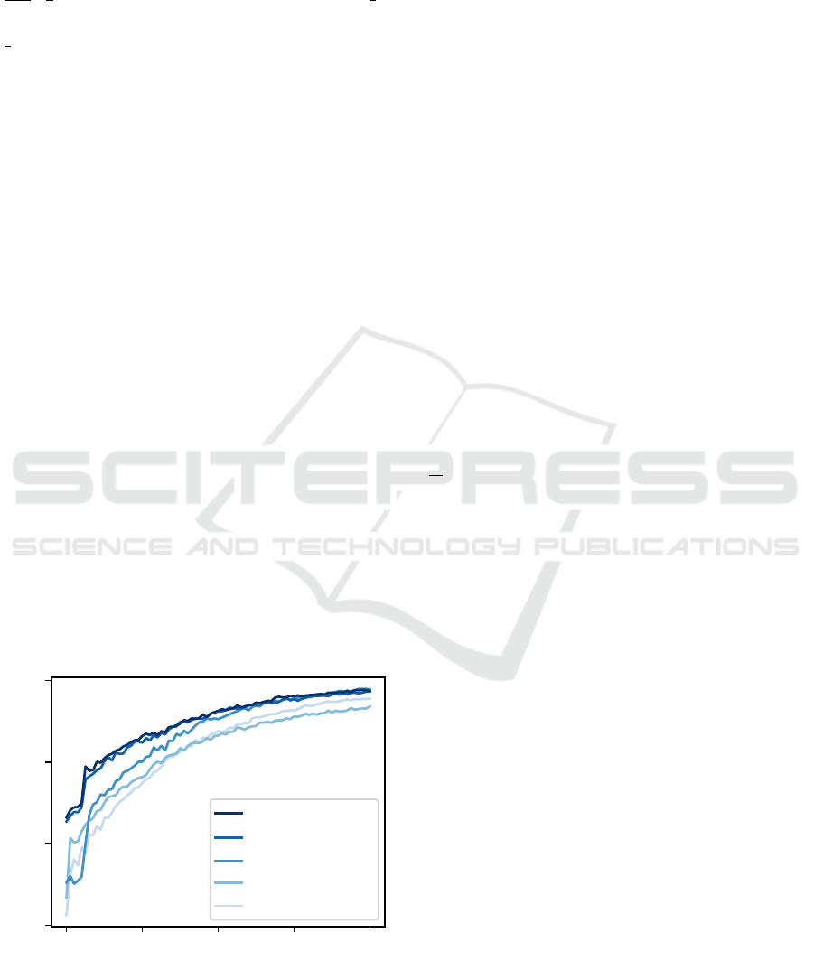
5.2 Results

Figure 4 shows the progress of the optimization of

the VQE and WS-VQE with different optimizer con-

ﬁgurations as stipulated above. Evidently, utilizing

ACAE for the parameter initialization in WS-VQE

signiﬁcantly improves the median approximation

ratio over standard VQE. While the median ap-

proximation ratio after 20 iterations reaches just

above 0.3 for the VQE, the WS-VQE variant can

reach a median approximation ratio well above 0.5,

depending on the optimizer conﬁguration. The ﬁnal

median approximation ratios obtained with WS-VQE

are also above those of the standard VQE. Moreover,

the different optimizer conﬁgurations for WS-VQE

discussed above signiﬁcantly impact its performance.

As Figure 4 shows, WS-VQE optimized with ρ

VQE

reaches lower median approximation ratios than

standard VQE for a portion of the early iterations.

In contrast, WS-VQE/ρ

static

WS-VQE

, where COBYLA’s ρ

20 40 60 80 100

Iteration

0.3

0.5

0.7

0.9

Median approx. ratio

WS-VQE/%

dynamic

WS-VQE

WS-VQE/%

static

WS-VQE

WS-VQE/%

VQE

VQE/%

static

WS-VQE

VQE/%

VQE

Figure 4: Progress of the (WS-)VQE optimization: Median

approximation ratio after each iteration i ∈ {20,. . ., 100} for

the 500 problem instances (see Section 5.1.1) with different

initial step sizes ρ, as declared in Section 5.1.6.

parameter is halved, performs signiﬁcantly better up

until just above 65 iterations where it starts to overlap

with WS-VQE/ρ

VQE

. Median approximation ratios

obtained with WS-VQE/ρ

dynamic

WS-VQE

are above those

of all other variants until they also start to overlap

with WS-VQE/ρ

static

WS-VQE

in the 50th iteration. These

results conﬁrm our assumptions regarding different

optimizer settings for WS-VQE. However, the differ-

ences appear to fade as the optimization progresses.

Moreover, the results of VQE/ρ

static

WS-VQE

, which we

included for comparison, show that the advantages of

WS-VQE are not merely due to the optimizer setting.

5.3 Optimization Landscape Analysis

Next, we further analyze WS-VQE’s two-step opti-

mization by illustrating parts of the parameter space

for the variational optimization. The optimization

landscapes plotted in Figure 5 show expectation val-

ues and ﬁdelities in a random two-dimensional slice

of the parameter space of the Ansatz depicted in Fig-

ure 2. Values for parameters not annotated on the axes

were selected uniformly at random for each problem

instance. Expectation values and ﬁdelities, respec-

tively, were evaluated for each point of an equidistant

grid in the space [−π, π] × [−π,π] with a distance of

. The problem instances and approximate eigen-

vectors are identical to the ﬁrst three instances from

the experiments above (cf. Figure 4). The approxi-

mation ratios are 0.99, 0.86, and 0.76, respectively.

For each problem instance (rows in Figure 5), four

different properties are shown in the respective slice

of the parameter space (columns in Figure 5): (i) the

expectation value for VQE as per Equation (1), (ii) the

estimated ﬁdelity for ACAE as per Equation (6) of

the respective quantum state prepared by the Ansatz

to the approximate eigenvector ⃗v

appr.

, (iii) the actual

ﬁdelity of the quantum state to ⃗v

appr.

, and (iv) the

actual ﬁdelity of the quantum state to an optimal ref-

erence eigenvector⃗v

opt.

. As in the experiments above,

the VQE expectation values were computed from 200

shots per circuit, whereas the ﬁdelity was estimated

based on 400 snapshots. The circuits were executed

on a noiseless simulator, actual ﬁdelities were

determined based on state vector simulation in Qiskit.

Due to the construction of WS-VQE, the parame-

ters are optimized for the estimated ﬁdelity of ACAE

(second column) ﬁrst, before the optimization con-

tinues for the expectation value of VQE (ﬁrst col-

umn). Therefore, it is essential for WS-VQE that a

high ﬁdelity is observed in proximity to low expecta-

tion values. Figure 5 illustrates a proximity of the re-

spective extrema of both properties in the parameter

space, which depends on the quality of the approxi-

Warm-Starting the VQE with Approximate Complex Amplitude Encoding

−π

Problem 1

appr.

= 0.99

Expectation Value

(VQE)

Estimated Fidelity

appr.

(ACAE)

Actual Fidelity

appr.

Actual Fidelity

opt.

-6.0

3.41

0.56

0.0

0.48

0.0

0.45

0.01

−π

Problem 2

appr.

= 0.86

-9.96

6.44

0.42

0.0

0.28

0.0

0.38

0.0

−π 0 π

−π

Problem 3

appr.

= 0.76

−π 0 π

-9.18

6.05

0.52

0.0

0.42

0.0

0.22

0.0

Figure 5: Slices of the parameter space of VQE and ACAE (left) for three different problem instances as compared to the

actual ﬁdelity of the quantum states prepared by the Ansatz to the approximate and an optimal eigenvector of the instance,

⃗v

approx.

and ⃗v

opt.

, (right). Each line corresponds to a problem instance as described in Section 5.1.1 for which a random

two-dimensional slice of the full 18-dimensional parameter space of the Ansatz depicted in Figure 2 is plotted. The other

parameters were chosen uniformly at random from [−π,π]. Labels on the color bars indicate minimal and maximal values.

mation. For example, the minimal expectation value

for problem 1 appears at parameter values very close

to those of the maximum estimated and actual ﬁdelity

to the approximate eigenvector. Since the approxi-

mate eigenvectors for problems 2 and 3 are of lower

quality, the similarities appear to fade progressively.

Meanwhile, the actual ﬁdelity to an optimal eigenvec-

tor (rightmost column) appears to still exhibit its max-

imum at a similar location for problem 2. However,

since only one single optimal eigenvector is consid-

ered in the illustration of the landscapes, the extrema

of the ﬁdelity do not necessarily coincide with those

of VQE, as is the case for problem 3. We assume that

there are other optimal or near optimal eigenvectors

that make the minima of the expectation value appear

in a different position. In other words, the quantum

state of the ﬁdelity maximum for the speciﬁc optimal

eigenvector of problem 3 may have less inﬂuence on

the expectation value than other solutions. This is also

consistent with the state ﬁdelity to this eigenvector

reaching a maximum value of only 0.22, as compared

to higher values for the other problems.

One particularly noteworthy observation in Fig-

ure 5 is that all ﬁdelities have only one clearly pro-

nounced maximum in the respective two-dimensional

space (for estimated ﬁdelity: an area where high val-

ues concentrate). For this observation the periodicity

of the analyzed parameter space with a period of 2π,

due to the simple rotation gates of the ansatz, needs to

be taken into account. In contrast, the expectation val-

ues exhibit local minima. Together with a proximity

of ﬁdelity maxima for good approximate eigenvectors

and expectation minima, this indicates that WS-VQE

might be able to avoid local optima due to initial

parameter optimization based on estimated ﬁdelity.

5.4 Scalibility

To assess WS-VQE’s scalability, we repeated the ex-

periments of Section 5.2 for larger sizes of matrices

and with adjusted hyperparameters to account for the

larger problem instances. In particular, we generated

100 random 32 × 32 Hermitian matrices, i.e., matri-

ces with 1 024 entries each, with a sparsity of 90%,

increased N

snaps

to 800 and N

shots

to 400, and allowed

for 100 iterations in ACAE and 200 iterations in VQE

optimization. Also the circuit depth, i.e., repetitions

in the Ansatz, has been doubled from two to four.

In addition, the optimizer’s parameters have been up-

dated to ρ

′

VQE

π, ρ

′

static

WS-VQE

π, and

IQSOFT 2025 - 1st International Conference on Quantum Software

Table 1: Median ﬁnal approximation ratio for 100 random

32 × 32 problem instances reached after a maximum of 200

VQE iterations, including ACAE pretraining for WS-VQE,

as described in Section 5.1.4.

Variant

Conﬁg.

′

VQE

′

static

WS-VQE

′

dynamic

WS-VQE

VQE 0.518 0.481 -

WS-VQE 0.530 0.507 0.548

′

dynamic

WS-VQE

π. The approximate eigenvector was

(12)

for the warm-start as per Equation (7).

The results are summarized by median ﬁnal ap-

proximation ratios for each variant’s parameteriza-

tion presented in Table 1. These results indicate that

the advantage of the warm-start persists also with in-

creasing problem instances. In particular, WS-VQE

reached higher approximation ratios for both values

of the initial step size parameter ρ. Also the dynamic

initial step size persisted as the most beneﬁcial regime

for setting this hyperparameter in WS-VQE. How-

ever, the results in Table 1 indicate that further ad-

justment of ρ may be needed, since the decrease from

′

VQE

to ρ

′

static

WS-VQE

lead to a reduced approximation

ratio in both cases and the overall performance de-

creased signiﬁcantly compared to the results of Sec-

tion 5.2, although the resources have been increased.

6 DISCUSSION

The evaluation shows that WS-VQE can be worth-

while, but a few caveats remain to be discussed.

6.1 Quality of the Approximation

Clearly, the success of WS-VQE depends on the qual-

ity of the approximations fed to the algorithm. On av-

erage, the approximations corresponded to an approx-

imation ratio around 0.850 (σ = 0.126) in our evalu-

ation in Section 5.2 and 0.911 (σ = 0.052) in Sec-

tion 5.4. We utilized a simple, but not generally fea-

sible approximation for eigenvectors, as the inverse

power method requires matrix inversion or solving

linear systems of equations, which incur a cost of cu-

bic complexity similar to that of the eigenvalue prob-

lem itself (Pan and Chen, 1999). Therefore, it would

be desirable to utilize more efﬁcient approximations.

These could be obtained, e.g., from previous solu-

tions of periodically recurring problems with only lit-

tle changes to the matrix, which are well-conditioned

according to the Bauer-Fike theorem (Bauer and Fike,

1960; Quarteroni et al., 2006). We emphasize that our

focus is on the warm-starting technique behind WS-

VQE; we do not intend to prove a quantum advantage.

6.2 Performance of ACAE

Another important factor in WS-VQE is the perfor-

mance of ACAE. In our evaluation, we observed

an average estimated ﬁdelity of 0.625 (σ = 0.230)

achieved within the 50 ACAE iterations in Section 5.2

and 0.197 (σ = 0.097) within the 100 ACAE itera-

tions in Section 5.4. Although the approximations

obtained from the inverse power method were of rel-

atively high quality, the low average ﬁdelity indi-

cates that ACAE was hardly able to retain this qual-

ity in its encoding. Despite the seemingly low ﬁ-

delity, WS-VQE still surpassed the performance of

standard VQE. However, another allocation of quan-

tum resources for ACAE and WS-VQE, respectively,

in particular providing more resources for the opti-

mization of ACAE, could yield a higher ﬁdelity and,

thus, better results. Moreover, further adjustment of

ACAE and its hyperparameters may be needed to im-

prove the quality of the encoding.

6.3 Expressivity of the Ansatz

An important prerequisite of the VQE is an Ansatz

that is tunable to prepare the desired optimal solu-

tion. This translates to the requirements of expressiv-

ity and trainability, i.e., the Ansatz needs to be expres-

sive enough to capture the optimal solution, but sim-

ple enough that its parameter space can be traversed

by the optimizer to reach an optimum (Funcke et al.,

2021; Du et al., 2022). Likewise, the ACAE requires

an expressive and trainable Ansatz for the encoding

of complex amplitudes. Although the Ans

atze for the

VQE and ACAE in principle need not be identical,

WS-VQE implicitly assumes that an Ansatz for the

VQE is also suitable to encode an approximate eigen-

vector with ACAE. This assumption appears reason-

able, particularly since ACAE only aims for an ap-

proximate encoding. Provided that the VQE Ansatz

is expressive, i.e., able to capture the optimum, and

trainable, which entails the ability to reach states “sur-

rounding” the optimum during the optimization to-

ward it, and that the approximate solution ⃗v is sufﬁ-

ciently close to the optimal solution, the same Ansatz

should also sufﬁce to approximately encode⃗v.

6.4 Choice of Classical Optimizers

The choice of the classical optimizer in VQE has sig-

niﬁcant impact on the efﬁciency and performance,

as it directly affects the number of measurements

and iterations required and can mitigate adverse ef-

fects (Tilly et al., 2022). Particularly, gradient-free

optimizers require signiﬁcantly fewer function eval-

Warm-Starting the VQE with Approximate Complex Amplitude Encoding

uations, as they omit evaluating points in the param-

eter space to compute gradients. For the evaluation,

we used the same gradient-free optimizer for both

ACAE and (WS-)VQE. However, it may be more

beneﬁcial to select different optimizers for each op-

timization, since the optimization landscapes of both

algorithms may exhibit different properties, as was il-

lustrated in Section 5.3. Moreover, some optimizers

are known to be more resilient to the noise on quan-

tum devices (Pellow-Jarman et al., 2021). Therefore,

different optimizers may be required when executing

(WS-)VQE on noisy quantum devices.

6.5 Mitigation of Adverse Effects

Parameter initializations have been shown to mitigate

adverse effects in the optimization of VQAs (Grant

et al., 2019; Lee et al., 2021). Particularly, barren

plateaus, i.e., areas with vanishing gradients in the pa-

rameter space of the cost function, and local minima

can be avoided with viable parameter initializations.

Thus, the convergence of VQAs may improve signif-

icantly when optimization is started closer to a global

optimum. We assume that the beneﬁts of WS-VQE

are partially due to the avoidance of adverse effects

by means of a viable parameter initialization. This

is supported by our analysis in Section 5.3, but addi-

tional evaluation is needed to quantify the mitigation.

6.6 VQE and Classical Shadows

As mentioned in Section 3, the idea of implement-

ing the VQE based on classical shadows has emerged.

WS-VQE also combines the VQE with classical shad-

ows, albeit differently. Additionally, WS-VQE is

fully compatible and complementary to a VQE imple-

mentation with classical shadows. Recall that ACAE

requires only an estimated ﬁdelity, that is obtained

with classical shadows from relatively few random

Clifford measurements. In contrast, the VQE may

still require a multitude of measurements even when

classical shadows are exploited, depending on the

Pauli composition of the operator (Tilly et al., 2022).

Hence, WS-VQE with ACAE pretraining could still

be more cost-efﬁcient than starting a VQE implemen-

tation with classical shadows from scratch.

6.7 Reuse of Clifford Unitaries

As mentioned in Section 5.1.4, we reduced the clas-

sical effort of the Clifford measurements in ACAE

by reusing the unitaries for the classical snapshots

throughout an optimization. Using the same unitaries

for ﬁdelity estimations throughout the optimization

could lead to overﬁtting, i.e., the model could learn

to accommodate the selected set of unitaries instead

of actually improving the state ﬁdelity. On the other

hand, changing the unitaries in each iteration may in-

crease the perturbation of the ﬁdelity estimation, mak-

ing the optimization more vulnerable. However, we

used relatively many snapshots, which mitigates both

potential problems to a certain extent. Moreover, our

results indicate that the ﬁdelity and encoding achieved

by ACAE was sufﬁcient to retain WS-VQE’s perfor-

mance beneﬁt. As an alternative, the random Clifford

unitaries could be sampled from a reduced set that ef-

fectively preserves the original quantum channel in-

troduced in Section 2.2, thus reducing the sampling

and compilation costs (Zhang et al., 2024).

6.8 Iterations and Queuing Times

Despite potentially recuding the total number of shots

needed, WS-VQE increases the total number of iter-

ations due to the pretraining. Since quantum com-

puters are often available as shared resources through

cloud services (Leymann et al., 2020; Vietz et al.,

2021), queueing times for quantum circuit execution

could increase with the number of iterations. Appro-

priate execution patterns supported by quantum cloud

service providers mitigate this drawback by enabling

prioritized execution of VQAs, removing the need to

wait in queues for every iteration (Georg et al., 2023).

7 SUMMARY AND OUTLOOK

In this work, we proposed a warm-starting technique

for the VQE that utilizes classical shadows. In partic-

ular, the warm-start is based on an approximate am-

plitude encoding of an approximate solution for the

problem at hand. The proposed technique enables uti-

lizing any given approximation of the problem that

determines an (approximate) eigenvector to generate

a beneﬁcial parameter initialization for the VQE. WS-

VQE is also compatible with different variants and

improvements of the VQE, as it does not require any

changes of the original algorithm or its quantum cir-

cuit. As shown in the evaluation, the VQE beneﬁts

from the warm-start in terms of a reduced quantum

computational effort needed to reach a certain solu-

tion quality. In addition, the evaluation showed that

adjusting the optimizer used in WS-VQE can fur-

ther improve the performance. As an auxiliary result,

we outlined a way to derive a parameter initializa-

tion from a biased initial state, which may serve as

a blueprint for warm-starting other VQAs.

For future work, it remains to evaluate WS-VQE

IQSOFT 2025 - 1st International Conference on Quantum Software

in more detail and with real-world use cases to de-

termine which applications could beneﬁt from it.

As Section 6 explained, changes in conﬁguration

and implementation could further improve the warm-

starting technique. Moreover, we aim to analyze

which other VQAs could beneﬁt from this technique

or adaptations. Furthermore, the Quokka ecosys-

tem (Beisel et al., 2023) could be extended to in-

tegrate WS-VQE-like warm-starts. The Quokka’s

warm-starting service currently facilitates the clas-

sical precomputation of parameter initializations and

biased initial states, which could be extended for WS-

VQE’s hybrid quantum-classical pretraining.

ACKNOWLEDGMENTS

This work was partially funded by the BMWK

projects SeQuenC (01MQ22009B) and EniQmA

(01MQ22007B).

REFERENCES

Barkoutsos, P. K., Gkritsis, F., Ollitrault, P. J., Sokolov,

I. O., Woerner, S., and Tavernelli, I. (2021). Quan-

tum algorithm for alchemical optimization in material

design. Chemical science, 12(12):4345–4352.

Bauer, F. L. and Fike, C. T. (1960). Norms and exclusion

theorems. Numer. Math., 2(1):137–141.

Beisel, M., Barzen, J., Garhofer, S., Leymann, F., Truger,

F., Weder, B., et al. (2023). Quokka: A Service

Ecosystem for Workﬂow-Based Execution of Vari-

ational Quantum Algorithms. In Service-Oriented

Computing – ICSOC 2022 Workshops. Springer.

Bernal, D. E., Ajagekar, A., Harwood, S. M., Stober, S. T.,

Trenev, D., and You, F. (2022). Perspectives of quan-

tum computing for chemical engineering. AIChE

Journal, 68(6).

Bravyi, S. and Maslov, D. (2021). Hadamard-free circuits

expose the structure of the clifford group. IEEE Trans-

actions on Information Theory, 67(7):4546–4563.

Cerezo, M., Arrasmith, A., Babbush, R., Benjamin, S. C.,

Endo, S., Fujii, K., et al. (2021). Variational quantum

algorithms. Nature Reviews Physics, 3(9):625–644.

Cervera-Lierta, A., Kottmann, J. S., and Aspuru-Guzik, A.

(2021). Meta-variational quantum eigensolver: Learn-

ing energy proﬁles of parameterized hamiltonians for

quantum simulation. PRX Quantum, 2(2).

Dborin, J., Barratt, F., Wimalaweera, V., Wright, L., and

Green, A. G. (2022). Matrix product state pre-training

for quantum machine learning. Quantum Science and

Technology, 7(3).

Du, Y., Tu, Z., Yuan, X., and Tao, D. (2022). Efﬁcient mea-

sure for the expressivity of variational quantum algo-

rithms. Phys. Rev. Lett., 128.

Egger, D. J., Mare

cek, J., and Woerner, S. (2021). Warm-

starting quantum optimization. Quantum, 5.

Feynman, R. P. (1982). Simulating physics with computers.

International Journal of Theoretical Physics, 21(6/7).

Funcke, L., Hartung, T., Jansen, K., K

uhn, S., and Stornati,

P. (2021). Dimensional expressivity analysis of para-

metric quantum circuits. Quantum, 5.

Galda, A., Liu, X., Lykov, D., Alexeev, Y., and Safro,

I. (2021). Transferability of optimal QAOA pa-

rameters between random graphs. In International

Conference on Quantum Computing and Engineering

(QCE), pages 171–180. IEEE.

Georg, D., Barzen, J., Beisel, M., Leymann, F., Obst, J.,

Vietz, D., et al. (2023). Execution Patterns for Quan-

tum Applications. In Proceedings of the 18

Inter-

national Conference on Software Technologies (IC-

SOFT). SciTePress.

Gershgorin, S. A. (1931).

Uber die Abgrenzung der Eigen-

werte einer Matrix. Bull. Acad. Sci. USSR, ser. VII,

7(6).

Grant, E., Wossnig, L., Ostaszewski, M., and Benedetti, M.

(2019). An initialization strategy for addressing bar-

ren plateaus in parametrized quantum circuits. Quan-

tum, 3.

Grimsley, H. R., Barron, G. S., Barnes, E., Economou, S. E.,

and Mayhall, N. J. (2023). Adaptive, problem-tailored

variational quantum eigensolver mitigates rough pa-

rameter landscapes and barren plateaus. npj Quantum

Information, 9(1).

Harwood, S. M., Trenev, D., Stober, S. T., Barkoutsos, P.,

Gujarati, T. P., Mostame, S., et al. (2022). Improving

the variational quantum eigensolver using variational

adiabatic quantum computing. ACM Transactions on

Quantum Computing, 3(1).

Head-Marsden, K., Flick, J., Ciccarino, C. J., and Narang,

P. (2021). Quantum information and algorithms

for correlated quantum matter. Chemical Reviews,

121(5):3061–3120.

Huang, H.-Y., Kueng, R., and Preskill, J. (2020). Predicting

many properties of a quantum system from very few

measurements. Nature Physics, 16(10):1050–1057.

Huang, H.-Y., Kueng, R., and Preskill, J. (2021). Efﬁcient

estimation of pauli observables by derandomization.

Phys. Rev. Lett., 127.

Kanno, S. and Tada, T. (2021). Many-body calculations for

periodic materials via restricted boltzmann machine-

based VQE. Quantum Science and Technology, 6(2).

Lee, X., Saito, Y., Cai, D., and Asai, N. (2021). Parameters

ﬁxing strategy for quantum approximate optimization

algorithm. In International Conference on Quantum

Computing and Engineering (QCE), pages 10–16.

Leymann, F. and Barzen, J. (2020). The bitter truth

about gate-based quantum algorithms in the NISQ era.

Quantum Science and Technology, pages 1–28.

Leymann, F., Barzen, J., Falkenthal, M., Vietz, D., Weder,

B., and Wild, K. (2020). Quantum in the Cloud: Ap-

plication Potentials and Research Opportunities. In

Proceedings of the 10

International Conference on

Cloud Computing and Services Science (CLOSER),

pages 9–24. SciTePress.

Warm-Starting the VQE with Approximate Complex Amplitude Encoding

Li, Y., Hu, J., Zhang, X.-M., Song, Z., and Yung, M.-H.

(2019). Variational quantum simulation for quantum

chemistry. Advanced Theory and Simulations, 2(4).

Mitarai, K., Suzuki, Y., Mizukami, W., Nakagawa, Y. O.,

and Fujii, K. (2022). Quadratic clifford expansion

for efﬁcient benchmarking and initialization of vari-

ational quantum algorithms. Physical Review Re-

search, 4(3).

Mitsuda, N., Ichimura, T., Nakaji, K., Suzuki, Y., Tanaka,

T., Raymond, R., et al. (2024). Approximate complex

amplitude encoding algorithm and its application to

data classiﬁcation problems. Phys. Rev. A, 109.

Mustafa, H., Morapakula, S. N., Jain, P., and Ganguly, S.

(2022). Variational quantum algorithms for chemical

simulation and drug discovery. In International Con-

ference on Trends in Quantum Computing and Emerg-

ing Business Technologies (TQCEBT), pages 1–8.

Nakaji, K., Uno, S., Suzuki, Y., Raymond, R., Onodera, T.,

Tanaka, T., et al. (2022). Approximate amplitude en-

coding in shallow parameterized quantum circuits and

its application to ﬁnancial market indicators. Physical

Review Research, 4(2).

Pan, V. Y. and Chen, Z. Q. (1999). The complexity of

the matrix eigenproblem. In Proceedings of the 31

Annual ACM Symposium on Theory of Computing,

STOC ’99, page 507–516, New York, NY, USA.

ACM.

Pellow-Jarman, A., Sinayskiy, I., Pillay, A., and Petruc-

cione, F. (2021). A comparison of various classi-

cal optimizers for a variational quantum linear solver.

Quantum Information Processing, 20(6).

Peruzzo, A., McClean, J., Shadbolt, P., Yung, M.-H., Zhou,

X.-Q., Love, P. J., et al. (2014). A variational eigen-

value solver on a photonic quantum processor. Nature

communications, 5(1):4213.

Powell, M. J. D. (1994). A Direct Search Optimiza-

tion Method That Models the Objective and Con-

straint Functions by Linear Interpolation, pages 51–

67. Springer Netherlands.

Preskill, J. (2018). Quantum computing in the NISQ era

and beyond. Quantum, 2.

Qiskit Contributors (2023). Qiskit: An open-source frame-

work for quantum computing.

Quarteroni, A., Sacco, R., and Saleri, F. (2006). Numerical

mathematics, volume 37. Springer Science & Busi-

ness Media.

Ravi, G. S., Gokhale, P., Ding, Y., Kirby, W., Smith, K.,

Baker, J. M., et al. (2022). CAFQA: A classical sim-

ulation bootstrap for variational quantum algorithms.

In Proceedings of the 28th ACM International Con-

ference on Architectural Support for Programming

Languages and Operating Systems (ASPLOS), page

15–29. ACM.

Rudolph, M. S., Miller, J., Motlagh, D., Chen, J., Acharya,

A., and Perdomo-Ortiz, A. (2023). Synergistic pre-

training of parametrized quantum circuits via tensor

networks. Nature Communications, 14(1).

Sack, S. H. and Serbyn, M. (2021). Quantum annealing ini-

tialization of the quantum approximate optimization

algorithm. quantum, 5.

Schuld, M. and Petruccione, F. (2018). Supervised learning

with quantum computers, volume 17. Springer.

Shaydulin, R., Lotshaw, P. C., Larson, J., Ostrowski, J., and

Humble, T. S. (2023). Parameter transfer for quantum

approximate optimization of weighted maxcut. ACM

Transactions on Quantum Computing, 4(3).

Shende, V., Bullock, S., and Markov, I. (2006). Syn-

thesis of quantum-logic circuits. IEEE Transactions

on Computer-Aided Design of Integrated Circuits and

Systems, 25(6):1000–1010.

Skogh, M., Leinonen, O., Lolur, P., and Rahm, M. (2023).

Accelerating variational quantum eigensolver conver-

gence using parameter transfer. Electronic Structure,

5(3).

Tao, Z., Wu, J., Xia, Q., and Li, Q. (2023). LAWS:

Look around and warm-start natural gradient descent

for quantum neural networks. In International Con-

ference on Quantum Software (QSW), pages 76–82.

IEEE.

Tate, R., Farhadi, M., Herold, C., Mohler, G., and Gupta,

S. (2023). Bridging classical and quantum with sdp

initialized warm-starts for qaoa. ACM Transactions

on Quantum Computing, 4(2).

Tilly, J., Chen, H., Cao, S., Picozzi, D., Setia, K., Li, Y.,

et al. (2022). The variational quantum eigensolver:

A review of methods and best practices. Physics Re-

ports, 986:1–128.

Truger, F., Barzen, J., Bechtold, M., Beisel, M., Leymann,

F., Mandl, A., et al. (2024). Warm-starting and quan-

tum computing: A systematic mapping study. ACM

Comput. Surv., 56(9).

Truger, F. and Obst, J. (2024). WS-VQE-prototype GitHub

Repository. https://github.com/UST-QuAntiL/

WS-VQE-prototype.

Verdon, G., Broughton, M., McClean, J. R., Sung, K. J.,

Babbush, R., Jiang, Z., et al. (2019). Learning to learn

with quantum neural networks via classical neural net-

works.

Vietz, D., Barzen, J., Leymann, F., Weder, B., and Yus-

supov, V. (2021). An Exploratory Study on the

Challenges of Engineering Quantum Applications in

the Cloud. In Proceedings of the 2

Quantum

Software Engineering and Technology Workshop (Q-

SET). CEUR Workshop Proceedings.

Wilson, M., Stromswold, R., Wudarski, F., Hadﬁeld, S.,

Tubman, N. M., and Rieffel, E. G. (2021). Optimiz-

ing quantum heuristics with meta-learning. Quantum

Machine Intelligence, 3:1–14.

Zhang, Q., Liu, Q., and Zhou, Y. (2024). Minimal-clifford

shadow estimation by mutually unbiased bases. Phys.

Rev. Appl., 21.

Zhang, Z.-J., Kyaw, T. H., Kottmann, J. S., Degroote, M.,

and Aspuru-Guzik, A. (2021). Mutual information-

assisted adaptive variational quantum eigensolver.

Quantum Science and Technology, 6(3).

IQSOFT 2025 - 1st International Conference on Quantum Software