TRIMARAN: A Toolbox for Radiometric Imaging with Microwave

ARrays of ANtennas

Eric Anterrieu

Centre d’

Etudes Spatiales de la BiOsph

ere (CESBiO),

Universit

e de Toulouse & CNRS-UMR5126, 18 avenue Edouard Belin, 31400 Toulouse, France

Keywords:

Antennas Arrays, Aperture Synthesis, Radiometry, Imaging.

Abstract:

This article aims at describing a Matlab toolbox named TRIMARAN intended to be used for Radiometric

Imaging with Microwave ARrays of ANtennas. Of course, only a few functions, the most important ones, out

of the 200 included in the toolbox are discussed and illustrated. In addition to this overview of TRIMARAN,

some concrete usages made by researchers, engineers or students are shown to illustrate the capabilities of this

toolbox. It has been used for designing aperture synthesis imaging radiometers and for quantifying instrument

performances as well as for discovering and for learning many aspects of microwave remote sensing by aper-

ture synthesis with realism.

1 INTRODUCTION

Aperture synthesis (Brouw, 1975) is a technique

that mixes the signals kept by a collection of ele-

mentary antennas (Christiansen and H

ogbom, 1987)

to produce images having the same angular resolu-

tion as that obtained with an instrument the size of

the entire collection. It has been used successfully

in radio astronomy since the 1950s (VLA, VLBI,

VLBA. . . ) (Thompson et al., 1980; Cohen, 1973;

Napier et al., 1994) as well as in Earth remote sensing

from space since the 1990s (ESTAR, SMOS. . . ) (Vine

et al., 1994; Barr

e et al., 2008; McMullan et al.,

2008). Unlike total power radiometers that point ac-

curately in many directions to measure the antenna

temperature and thus compose a brightness temper-

ature map, aperture synthesis imaging radiometers

combine the signals kept by every elementary an-

tenna, electronically or numerically, in order to pro-

duce a brightness temperature map with the aid of a

computer. There are two ways to combine these el-

ementary signals, known as multiplicative synthesis

and additive synthesis. The former combines these

antennas signals by pairs in a cross-correlator to per-

form synthetic aperture interferometry, whereas the

latter mixes them all together to operate digital beam

forming (Anterrieu et al., 2022).

TRIMARAN is a Matlab (The MathWorks, a)

https://orcid.org/0009-0007-2233-9098

toolbox that offers users the opportunity to play nu-

merically with both paradigms on the simulation of

the radio signals kept by each elementary antenna

and on their combination to produce either complex

visibilities (multiplication synthesis in interferome-

try) or antenna array maps (additive synthesis with

beam forming). It is able to process them with up-to-

date regularized inversion methods for retrieving the

brightness temperature distribution of the scene un-

der observation. For both approaches, TRIMARAN

is capable of simulating data and of inverting them

for an observed scene in the far-ﬁeld region of the an-

tenna array as well as in the near-ﬁeld zone (Anterrieu

et al., 2024), in ground based as well as in airborne or

spaceborne situations. In every case TRIMARAN can

also digest real data from an actual instrument. More-

over, as an open-source software subject to evolutions

and to improvements, it will be able to process real

data from future instruments like it does today with

SMOS.

From a practical point of view, TRIMARAN is

a self-sufﬁcient collection (no additional toolbox re-

quired) of about 200 Matlab functions written in ac-

cordance with the MathWorks programming stan-

dards. They are divided into 9 thematic groups (or-

bitography, antenna array, antenna patterns, ﬁeld of

view, instrument modeling, radio signals, brightness

temperature maps, graphic and others) that are brieﬂy

presented with illustrations in section 2. TRIMARAN

relies on multidisciplinary knowledge (microwave ra-

242

Anterrieu, E.

TRIMARAN: A Toolbox for Radiometric Imaging with Microwave ARrays of ANtennas.

DOI: 10.5220/0013503700003970

In Proceedings of the 15th International Conference on Simulation and Modeling Methodologies, Technologies and Applications (SIMULTECH 2025), pages 242-253

ISBN: 978-989-758-759-7; ISSN: 2184-2841

diometry, antenna theory, applied mathematics, sig-

nal & image processing). It is intended for, and it is

used by, students at master science level for discover-

ing playfully and for learning rigorously many aspects

of microwave remote sensing by aperture synthesis

with realism. It is also meant for, and used by, en-

gineers from space industry and agencies for quickly

designing aperture synthesis imaging radiometers and

for practically quantifying instrument performances.

It has been operated recently by researchers for sim-

ulating a huge dataset to implement and to evaluate

the performances of a deep learning approach for the

inversion of the complex visibilities provided by the

imaging radiometer MIRAS onboard the SMOS mis-

sion of the European Space Agency (ESA). Some of

these concrete usages are shown in section 3 to illus-

trate the capabilities of TRIMARAN.

2 FUNCTIONS OVERVIEW

As outlined in the introduction, TRIMARAN is a col-

lection of about 200 Matlab functions (for ease of

reading, all elements of the Matlab language are writ-

ten here in blue with a ﬁxed font). Of course, only

few of these functions are discussed or illustrated in

this section. For the others, the user is invited to dis-

cover them with the lookfor facility and with the

in-line examples accessible from the help command.

Indeed, all the functions of TRIMARAN meet Math-

Works programming standards and for most of them

an additional section of the in-line help entitled “Ex-

ample” has been added in order to provide the user

with illustrating usages of the function, while waiting

for a user guide to be written!

2.1 Orbitography

The function CircularOrbit returns the orbital pe-

riod T and the orbital velocity v for a circular orbit

at a given elevation h around the Earth. If h lies in

an appropriate range, it also returns the required in-

clination i for a sun-synchronous orbit, otheriwse 90

◦

is returned and the orbit is a polar one. For the SMOS

mission, these elements are:

> h=771E+03;

> [i,T,v]=CircularOrbit(h)

i = 98.4526

T = 6.0068e+03

v = 7.4707e+03

Although this modeling is very basic, it is sufﬁ-

cient to conduct pre-studies and if necessary it can be

replaced by a ﬁner model. As a comparison between

this circular orbit approximation and the most up-

to-date orbital mechanics codes used by CNES and

ESA (Barr

e et al., 2008), with an average elevation of

771 Km the ofﬁcial orbital period of SMOS is given

for 6004.5 s and its inclination for 98.445

◦

, whereas

they are estimated here around 6006.8 s and 98.453

◦

respectively.

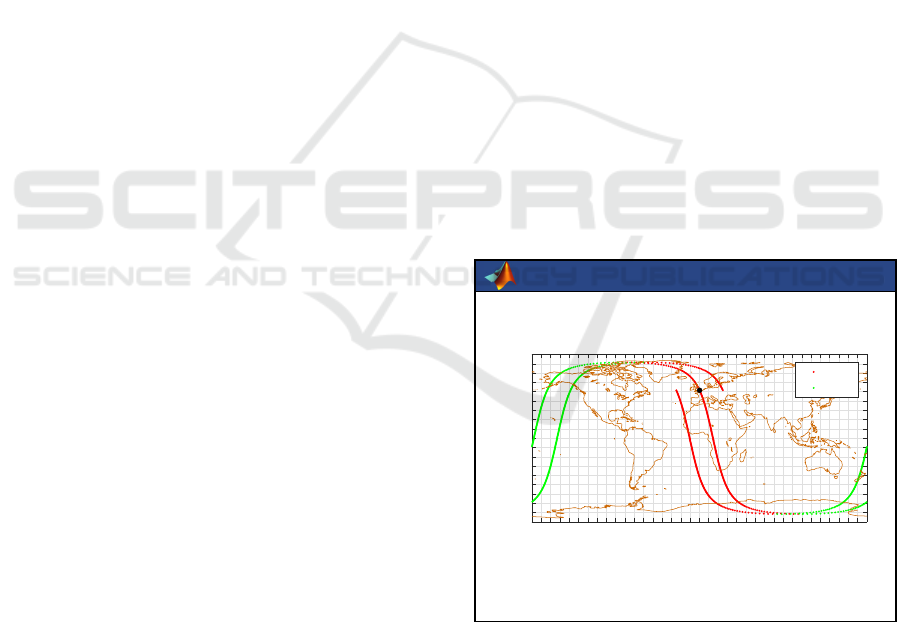
The function CircularOrbitPropagate is a

forward-backward orbit propagator that returns the

geographic coordinates (Chang, 2016) at given dates t

starting from a given location at t = 0. It also returns

the direction of the passes (ascending or descending).

Hereafter are the few lines to calculate two circular

orbits passing over London:

> LatS=dms2deg(51,30,26);

> LonS=dms2deg( 0, 7,39);

> [Lon,Lat,pass]= ...

CircularOrbitPropagate(h,i,’Asc’, ...

LonS,LatS,linspace(-T,T,1000));

> Asc=strfind(pass,’A’);

> Dsc=strfind(pass,’D’);

> figure;plot(Lon(Asc),Lat(Asc),’r.’, ...

Lon(Dsc),Lat(Dsc),’g.’);

> geoplotWORLD;

> legend(’Asc’,’Dsc’);

The geographic coordinates returned in Lat and

Lon are plotted on Figure 1 together with the world’s

costlines drawn with the function geoplotWORLD.

TRIMARAN

180°W 90°W 0° 90°E 180°E

90°S

60°S

30°S

0°

30°N

60°N

90°N

Asc

Dsc

Figure 1: Example of ascending (red) and descending

(green) circular orbits passing over London (black dot), as

returned by the function CircularOrbitPropagate.

2.2 Antenna Array

The function AntennaArray returns the coordinates

of the elementary antennas, the antennas pairs of ev-

ery baseline, the components of the baselines and

TRIMARAN: A Toolbox for Radiometric Imaging with Microwave ARrays of ANtennas

243

the corresponding Fourier frequencies with their re-

dundancy. . . . Many geometries (circle, octagon,

hexagon, square, triangle, cross, Y) are available for

any number of elementary antennas regularly spaced

with a short spacing d and operating at a central wave-

length λ

. As the guiding thread of this presentation

is the SMOS mission operating in the B

= 20 MHz

protected band centered on f

= 1413.5 MHz, param-

eters of the MIRAS antenna array are available from

the high-level function SMOSarray:

> Bo=20E+06;

> Fo=1413.5E+06; Lo=299792458/Fo;

> d=0.875;

> [˜,˜,Xa,Ya,cal,˜,P,Q,˜,˜,Ub,Vb, ...

˜,˜,˜,Uf,Vf,Rf]=SMOSarray(90,d,Lo);

> figure;plotAA(Xa,Ya,cal);

> figure;plotFF(Uf*Lo,Vf*Lo,Rf);

The antenna array of MIRAS with its 69 elemen-

tary antennas regularly spaced with d = 0.875λ

the three arms of a (rotated) Y is shown on Figure 2

where the cartesian coordinates Xa and Ya are re-

ported. The corresponding uv-coverage is shown on

Figure 3 where the Fourier frequencies Uf and Vf are

plotted with a color indicating the redundancy Rf.

TRIMARAN

-4 -2 0 2

-3

-2

-1

[m]

Figure 2: MIRAS, the antenna array of the SMOS space

mission with 69 elementary antennas, as plotted by the

function plotAA (those in green are used for calibration pur-

pose). The shortest spacing is d = 0.875λ

≃ 18.6 cm and

the longest baseline is 21

√

3d ≃ 6.75 m.

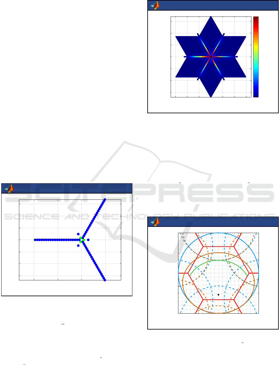
2.3 Field of View

The paired functions plotFOV cart and

plotFOV hexa plot the ﬁeld of view at instru-

ment level where aperture synthesis takes place.

For the MIRAS instrument onboard SMOS that is

tilted forwardly from the Nadir direction with an

TRIMARAN

-6 -4 -2 0 2 4 6

-6

-4

-2

redundancy

U [m]

V [m]

Figure 3: The uv-coverage of MIRAS with its 2791 Fourier

frequencies, as plotted by the function plotFF. The redun-

dancy varies from 1 to 22 (for the shortest spacing).

angle ε = 31.2

◦

, the result is shown on Figure 4:

> tilt=32.5;

> figure;plotFOV_hexa(h,tilt,d,90,60.6);

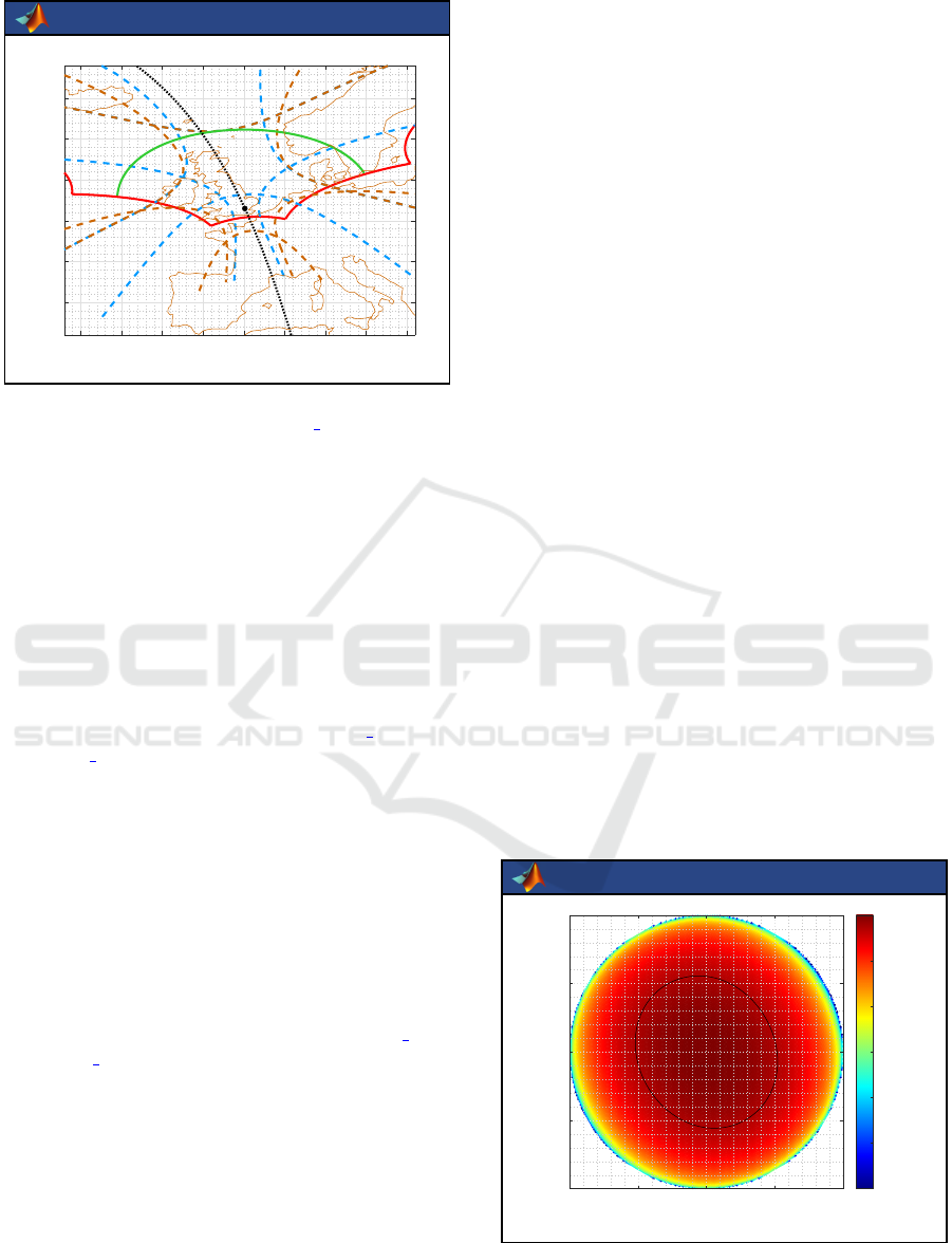
Likewise, the twinned functions

geoplotFOV cart and geoplotFOV hexa plot

the ﬁeld of view at ground level, as shown on

Figure 5:

> figure;geoplotFOV_hexa(h,i,’Asc’, ...

TRIMARAN

-1 -0.5 0 0.5 1

-1

-0.5

0.5

= sinθcosφ

= sinθsinφ

Figure 4: Hexagonal ﬁeld of view of SMOS at instrument

level, as plotted by the function plotFOV hexa. Here the

MIRAS antenna array is subject to ﬁeld aliasing because of

the spacing between the elementary antennas: the hexag-

onal ﬁeld of view and its six neighbors are drawn in red,

the Earth and its aliases are drawn in maroon, the sky and

its aliases are drawn in blue, the ground incidence 60.6

◦

drawn in green, the black dot is the sub-satellite point with

coordinates (0,−sinε).

SIMULTECH 2025 - 15th International Conference on Simulation and Modeling Methodologies, Technologies and Applications

244

TRIMARAN

20°W 10°W 0° 10°E 20°E

40°N

50°N

60°N

Figure 5: Hexagonal ﬁeld of view of SMOS at ground level,

as plotted by the function geoplotFOV hexa. Referring

back to Figure 4, here the sub-satellite point (black dot) is

geo-localized over London and the ascending pass (black

dotted curve) is that of a sun-synchronous circular orbit.

tilt,d,90,LonS,LatS,60.6);

When designing an aperture synthesis imaging ra-

diometer, these functions are very useful for making

the required trade-off between various ﬁgures of merit

that may depend from several parameters like the el-

evation h, the geometry of the antenna array and the

spacing d as well as the tilt angle ε. . . This is the case,

for example, of the useful ground swath that is re-

turned by the twinned functions swathFOV cart and

swathFOV hexa which has, together with the orbital

period T , a direct impact on the revisit time:

> swath=swathFOV_hexa(h,i,’Asc’, ...

tilt,d,90,LonS,LatS)

swath = 1.4330e+06

In that case of SMOS, 1433 Km with an orbital

period of 100 min is fully compatible with a revisit

time of 3 days at the equator.

Finally, aperture synthesis is performed at instru-

ment level with the aid of the computer. As a conse-

quence, sampling grids are required for discretizing

integral equations. The two functions grids cart

and grids hexa return the values taken by the direc-

tions cosines and by the spherical angles over sam-

pling grids as well as many other quantities:

> N = 128;

> [˜,˜,X,Y,Sxy,˜,Theta,Phi]= ...

grids_hexa(h,tilt,d,90,N);

Theta and Phi are 1×2 cell arrays with the spher-

ical angles θ and φ, respectively. X and Y are also 1×2

cell arrays with the components of ξ: ξ

= sin θcos φ

and ξ

= sin θsin φ, respectively. Sxy is the elemen-

tary area dξ of a pixel in the corresponding sampling

grid. For every 1×2 cell array, the ﬁrst element {1}is

a N×N array limited to the ﬁeld of view synthesized

by the antenna array whereas the second one {2} is

a 2N ×2N array with the corresponding quantity in

the space 0 ≤ θ ≤ π/2 and 0 ≤ φ ≤ 2π in front of the

instrument. Among the other quantities returned by

these two functions, very useful ones are the indices

of the pixels from the grids X and Y that belong to the

Earth or to the sky in the ﬁeld of view, returned in

1×2 cell arrays PXLearth and PXLsky.

2.4 Antenna Patterns

Elementary antenna patterns are at the heart of anten-

nas arrays. Although TRIMARAN is able to digest

any measured pattern, the AVP function returns a volt-

age pattern that follows a cos

θ law (Anterrieu et al.,

2003) with n related to the shape of the main beam:

> F{2}=AVP(Theta{2},Phi{2}-30,60,70);

> figure;plotAPP(X{2},Y{2},F{2},[-50 10]);

TRIMARAN has a family of functions

AVPestim* and APPestim* to estimate parameters of

voltage or power patterns like directivity D and equiv-

alent solid angle Ω as deﬁned by Equations (2–23)

and (2–24) in (Balanis, 2005), Full-Width at Half-

Maximum (FWHM). . . Hereafter are the lines to

estimate these ﬁgures of merit for the power pattern

of Figure 6:

> Omega=APPestimESA(F{2},[],X{2},Y{2},Sxy)

Omega = 12.5664

> D=APPestimDIR(F{2},[],X{2},Y{2},Sxy)

D = 10.0509

> FWHM=APPestimFWHM(F{2},X{2},Y{2})

TRIMARAN

-1 -0.5 0 0.5 1

-1

-0.5

0.5

-50

-40

-30

-20

-10

= sinθcosφ

= sinθsinφ

power pattern [dB]

Figure 6: An example of a power pattern |F (ξ)|

, as re-

turned by the function AVP and plotted by the function

plotAPP. Black ellipse is the half-maximum power contour.

TRIMARAN: A Toolbox for Radiometric Imaging with Microwave ARrays of ANtennas

245

FWHM = 70.0000 60.0000 -60.0000

2.5 Instrument Modeling

According to the Van-Cittert Zernike theorem (van

Cittert, 1934; Zernike, 1938) and referring to Figure7,

the theoretical complex visibility V

for a pair of el-

ementary antennas A

and A

in the far-ﬁeld approx-

imation is given by the relation:

Z Z

∥ξ∥≤1

(ξ)

Ω

∗

(ξ)

Ω

T (ξ)



−

·ξ



×e

−2jπ

·ξ

dξ

1 −∥ξ∥

(1)

where b

is the baseline vector between A

and A

the components ξ

= sinθ cos φ and ξ

= sinθ sin φ of

the angular position variable ξ are direction cosines

in the reference frame of the array, θ and φ are the

traditional spherical coordinates (the colatitude and

the azimuth, respectively), F

(ξ) and F

(ξ) are the

voltage patterns of the two elementary antennas with

equivalent solid angles Ω

and Ω

, T(ξ) is the bright-

ness temperature distribution of the scene under ob-

servation,

(t) is the so-called fringe-washing func-

tion which accounts for spatial decorrelation effects

for t = −b

·ξ/c and λ

= c/ f

is the central wave-

length of observation.

−r

θ θ

incident

wavefront

Figure 7: Two elementary antennas A

and A

pointing in

the same direction, here the Nadir as illustrated by the main

beam of the power patterns (in blue), r

and r

are location

vectors with respect to the far-ﬁeld source and the two an-

tennas are separated by the baseline vector b

The previous integral equation is implemented in

the function GT sai. Hereafter are the few lines to

obtain the 4695 complex visibilities of MIRAS corre-

sponding to an artiﬁcial scene that is set to a constant

temperature 100 K over Earth and 0 K elsewhere:

> T=zeros(2*N,2*N); T(PXLearth{2})=100;

> Vpq=GT_sai(Fo,Bo,F{2}./sqrt(Omega), ...

P,Q,Ub,Vb,[], ...

X{2},Y{2},Sxy,0,T);

> figure;plotVIS(Ub*Lo,Vb*Lo, ...

vis2vis(P,Q,Vpq),’abs’);

TRIMARAN

0 1 2 3 4 5 6 7

-3

-2

-1

| [m]

|V pq| [K]

Figure 8: Magnitude of the complex visibilities V

of a ﬂat

scene T

at a constant temperature 100 K, as plotted by the

function plotVIS.

Referring back to the sampling grids introduced

earlier in this section, after discretization of the inte-

gral found in (1) the relationship between the complex

visibilities and the brightness temperature distribution

of the scene under observation can be written in the

algebraic form:

V = GT (2)

where G is the linear modeling matrix of the imaging

radiometer returned by the function matG sai:

> G=matG_sai(Fo,Bo,F{1}./sqrt(Omega), ...

P,Q,Ub,Vb,[],X{1},Y{1},Sxy);

The inverse problem which aims at inverting rela-

tion (2) is ill-posed as a consequence of the rank de-

ﬁciency of G which is illustrated by the distribution

of its singular values, as shown in Figure 9 where two

groups are well separated by a large gap.

> rank(G)

ans = 2791

> svG=svd(G);

> [T,idxT]=getThresholdSV(svG,Uf,Vf)

T = 8.8343e-04

SIMULTECH 2025 - 15th International Conference on Simulation and Modeling Methodologies, Technologies and Applications

246

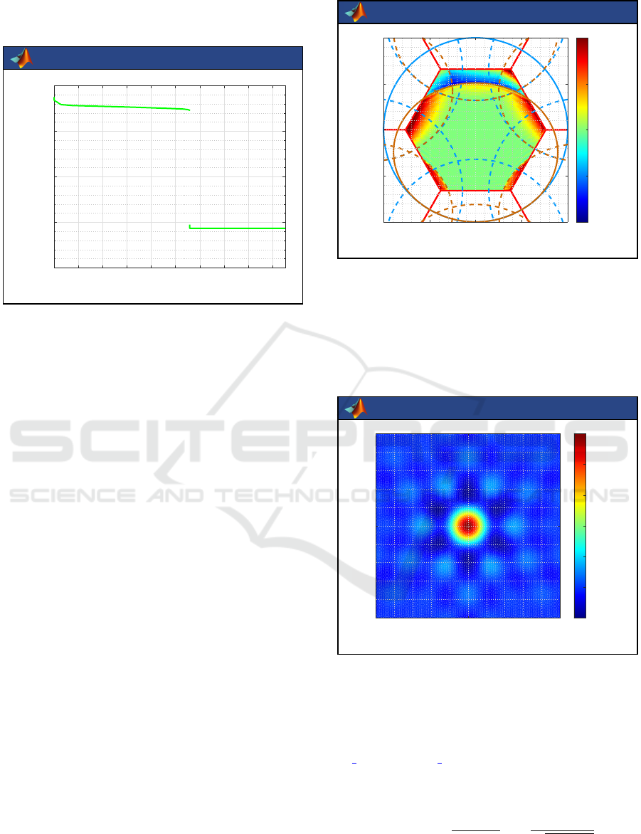
idxT = 2791 2792

> figure;plotSV(svG,[1 idxT(1)]);

TRIMARAN

0 1000 2000 3000 4000

-20

-15

-10

-5

index

singular values

Figure 9: Distribution of the singular values of the modeling

matrix G, as plotted by the function plotSV.

As a consequence, the smallest ones have to be

discarded prior the inversion to obtain a regularized

version of G

> Gp=pinv(G,T);

> Tr=reshape(Gp*Vpq,[N N]);

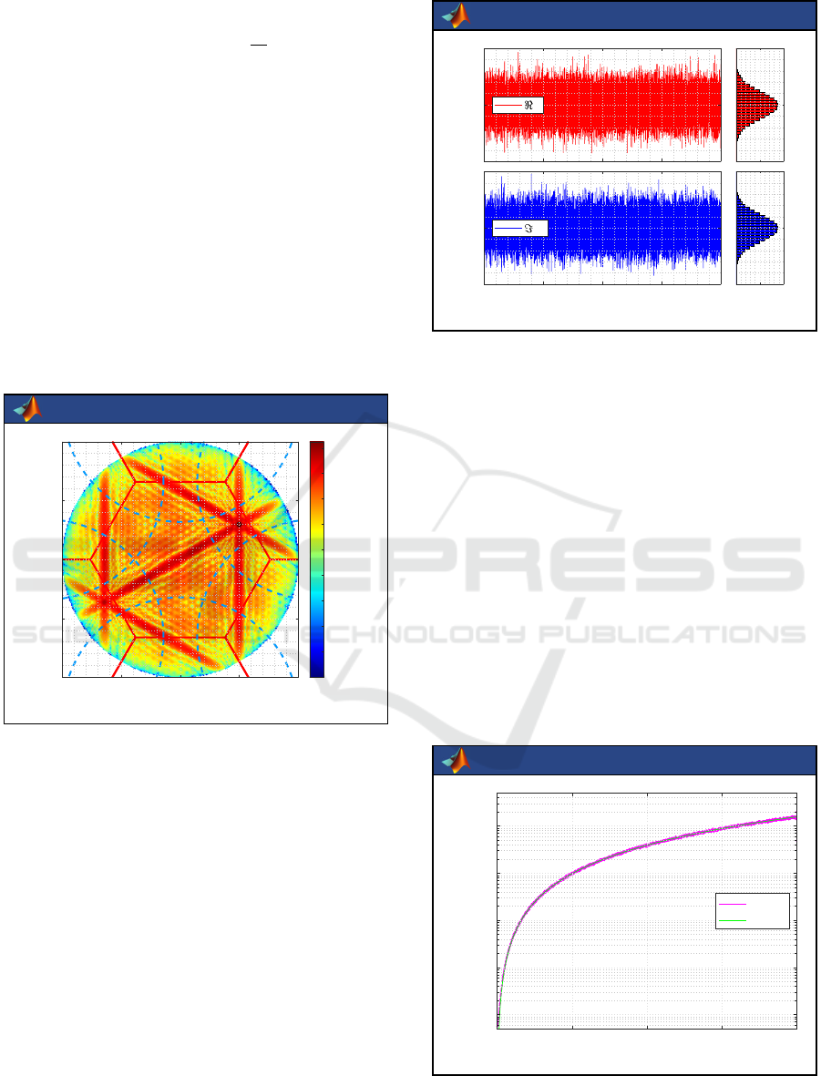
> figure;plotBTM(X{1},Y{1},Tr,[]);

> plotFOV_hexa(h,tilt,d,90,[]);

Shown on Figure 10 is the brightness temper-

ature T

= G

V thus obtained. TRIMARAN of-

fers alternative methods (Picard and Anterrieu, 2005)

to this popular truncated singular value decomposi-

tion (Goodberlet, 2000) among which the regularizing

approach implemented for SMOS (Anterrieu, 2004),

the Tikhonov one (Tikhonov and Arsenin, 1977) and

few total variation approaches (Chambolle, 2004).

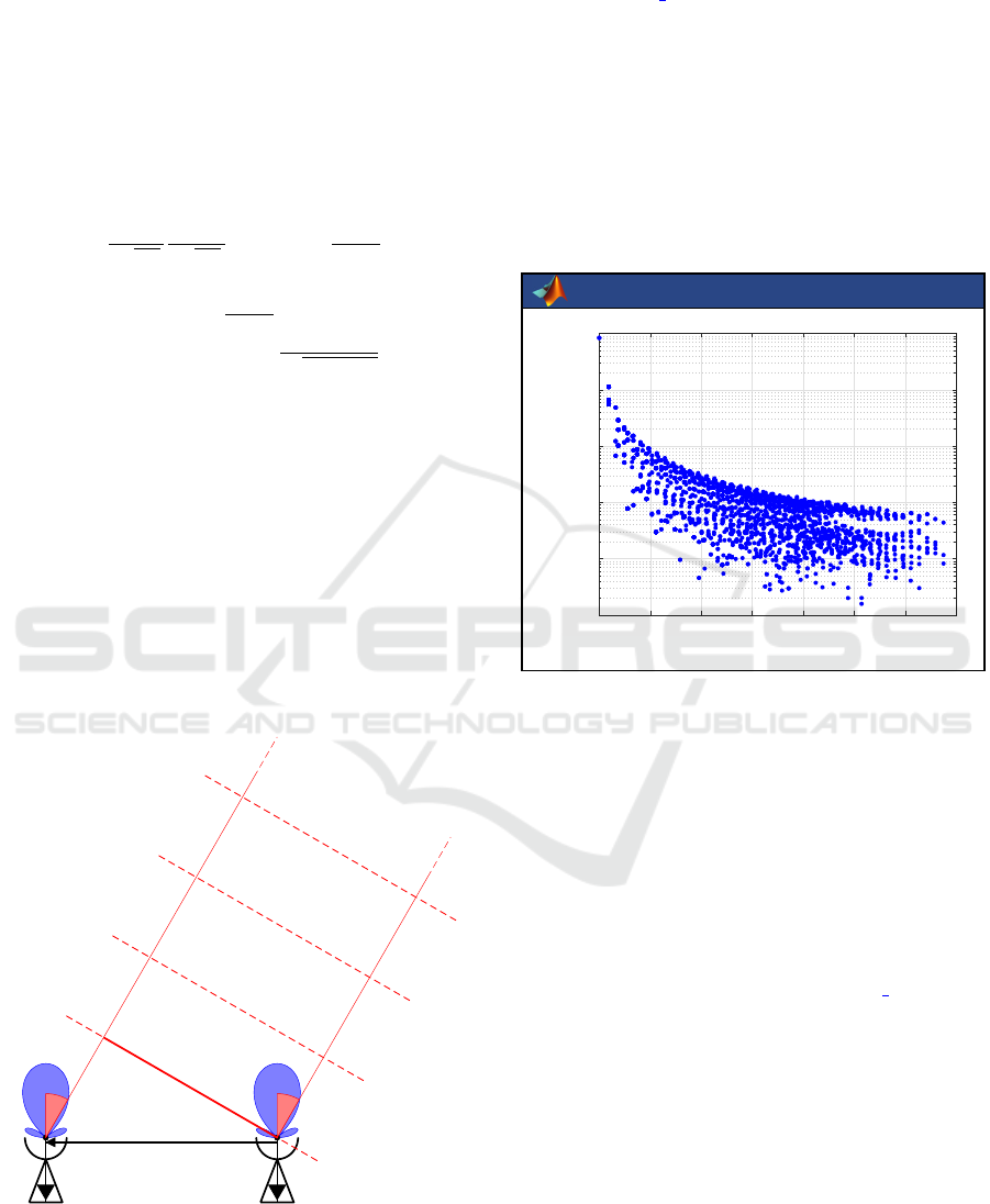
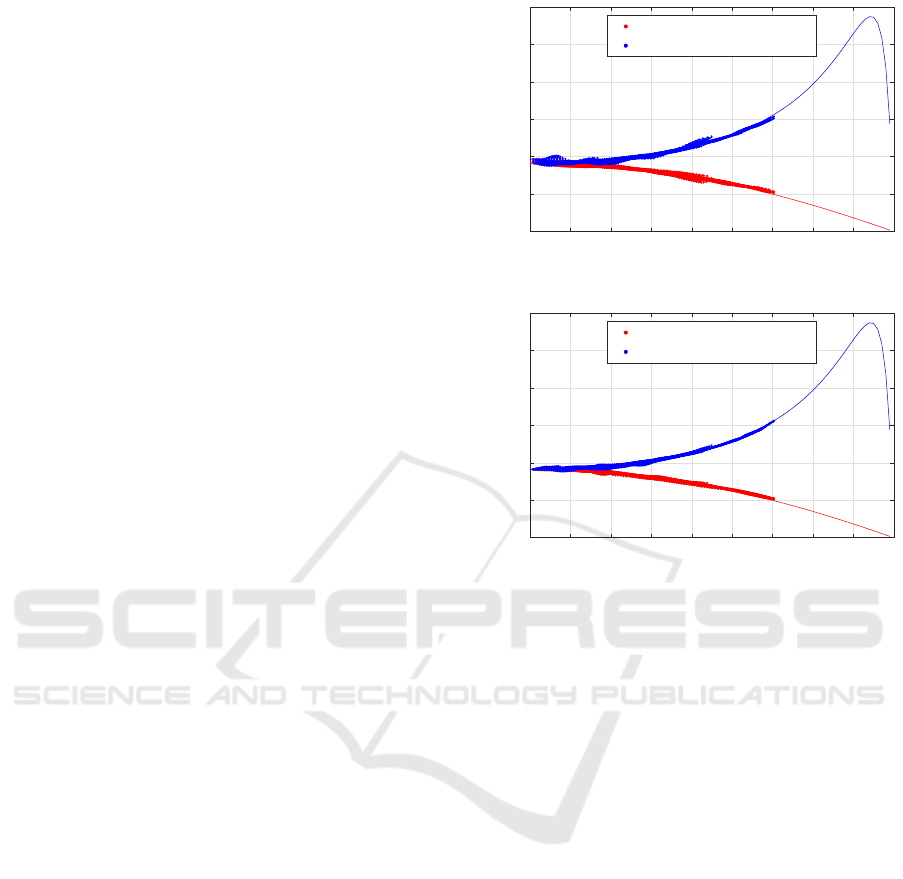
The same kind of simulation can be performed

but with the brightness temperature distribution of

a point source, so that the Point-Spread Function

(PSF) of the instrument can be estimated. This is

exactly what is done very simply by the function

PointSpreadFunction as shown on Figure11.

> PSF=PointSpreadFunction(Uf,Vf,N);

> figure;plotBTM(X{1},Y{1},PSF,[]);

> axis([-1 1 -1 1]*0.1);

The function ApodizationWindow returns an

apodization window that can be chosen among many

and apply to any brightness temperature map with the

aid of the function apodizeBTM. With regards to any

PSF, wether it is apodized or not, the two functions

AngularResolution and GroundResolution offer

facilities to estimate the angular resolution at instru-

TRIMARAN

-1 -0.5 0 0.5 1

-1

-0.5

0.5

100

150

200

= sinθcosφ

= sinθsinφ

brightness temperature [K]

Figure 10: Retrieved brightness temperature map T

V , as plotted by the function plotBTM. Referring back

to Figure 4, Earth aliases are clearly visible exactly where

they are supposed to be. In the Earth alias-free part, the re-

trieved temperature is the expected one.

ment level and the spatial one at ground level, respec-

tively.

TRIMARAN

-0.1 0 0.1

-0.1

0.1

-0.2

0.2

0.4

0.6

0.8

= sinθcosφ

= sinθsinφ

normalized PSF

Figure 11: Normalized PSF of MIRAS antenna array, as

plotted by the function plotBTM in the reduced domain

−0.1 ≤ ξ

≤ 0.1 and −0.1 ≤ξ

≤ 0.1.

Finally, additive synthesis with digital beam form-

ing is available in TRIMARAN with the functions

GT dbf and matG dbf which implement the integral

relation between T (ξ) and the antenna array tempera-

ture T(ξ

′

) from a direction ξ

′

T(ξ

′

) =

Z Z

∥ξ∥≤1

′

(ξ)|

Ω

′

T (ξ)

dξ

1 −∥ξ∥

, (3)

TRIMARAN: A Toolbox for Radiometric Imaging with Microwave ARrays of ANtennas

247

where

′

(ξ) =

∑

p=1

(ξ)e

−2jπ

(ξ −ξ

′

)

(4)

is the voltage pattern of the antenna array when point-

ing in the direction ξ

′

and with equivalent solid an-

gle Ω

′

. The antenna array patterns F

′

(ξ) are cal-

culated in the ArrayAVP function and their equiv-

alent solid angle Ω

′

is returned by the function

AVPestimESA. An example of F

′

(ξ) is shown on Fig-

ure 12. As expected, it is much narrower than the el-

ementary pattern F (ξ) shown in Figure 6 and more

directive as its directivity returned by APPestimDIR

is about 42.5 dB (this is equal to that of F (ξ), which

is about 10 dB, augmented by the number of elemen-

tary antennas (here M = 69 ≃ 36.8 dB) and reduced

by the attenuation F (ξ

′

)/F (0) ≃ −4.3 dB).

TRIMARAN

-1 -0.5 0 0.5 1

-1

-0.5

0.5

-50

-40

-30

-20

-10

= sinθcosφ

= sinθsinφ

power pattern [dB]

Figure 12: An example of antenna array power pat-

tern |F

′

(ξ)|

when pointing in the direction ξ

′

= (0.5, 0.3),

as returned by the function ArrayAVP and plotted by the

function plotAPP. Here again, referring back to Figure4,

aliases are where they are supposed to be, as illustrated by

the grating lobe in the direction ξ = (−0.64,−0.36).

2.6 Radio Signals

It is sometimes necessary to work at the level of

the signal kept by the elementary antennas (Anter-

rieu et al., 2017), particularly when the assumptions

accompanying the Van-Cittert Zernike theorem are

not satisﬁed. Although these calculations are time

consuming ones, thanks to GPU usage in functions

RadioSignal and RadioSignalCal, when such ac-

celerators are found on the computer and when the

Parallel Computing Toolbox (The MathWorks, b) is

available, computational time can be reduced down

to acceptable values, depending on the sampling fre-

TRIMARAN

-5

0 1 2 3 4

-5

0 5 10

t [µsec]

E(t) [mV/m]

[%]

Figure 13: First samples of a (complex-valued) radio signal

simulated by RadioSignal with f

= 8 GHz, as plotted by

the function plotEMF.

quency f

and on the duration T

of the signal to sim-

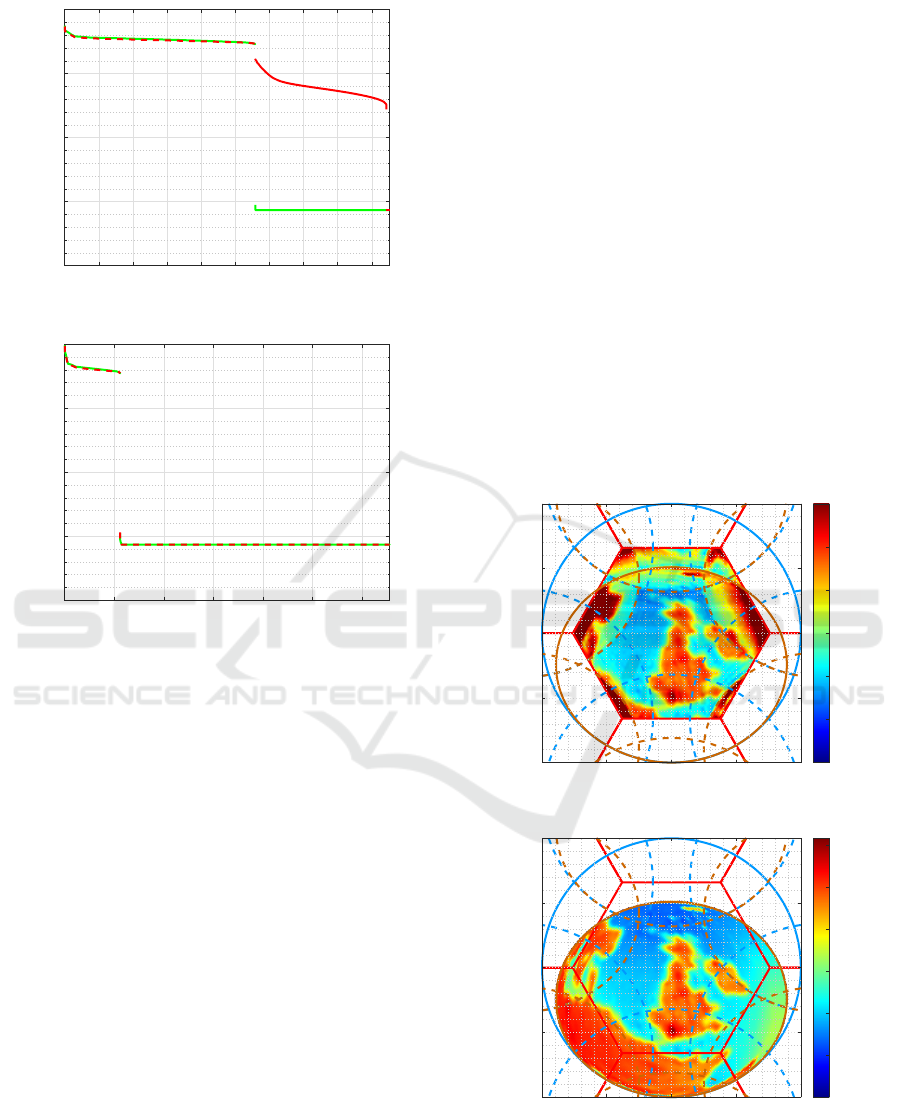
ulate. Shown on Figure 13 is an example of radio

signal kept by an element of MIRAS. As shown on

Figure 14 this signal is not just a white noise with a

Gaussian Probability Density Function (PDF) in the

time domain: its Power Spectral Density (PSD) in

the frequency domain is that of a black body at the

temperature of the scene (returned by the function

PlanckLaw), as expected. Accounting for this col-

oration of the spectrum (obtained with a FIR ﬁlter

returned by the function FirPlanckLaw) as well as

for the propagation times between each pixel of the

source and any antenna (evaluated by the function

FlyingTime) to take into account the Doppler effect,

explain the consequent calculation time for such sim-

TRIMARAN

0 1 2 3 4

-9

-8

-7

-6

-5

Planck

f [GHz]

( f ) [V

]

Figure 14: PSD of the radio signal shown on Figure 13, as

computed by the function PSDwelch and plotted with Mat-

lab’s function semilogy in the range 0 ≤ f ≤ f

/2.

SIMULTECH 2025 - 15th International Conference on Simulation and Modeling Methodologies, Technologies and Applications

248

ulations. When ﬁltering the signal of Figure 13 in

the B

= 20 MHz band centered on f

= 1413.5 MHz

(with an appropriate Raised-cosine ﬁlter calculated

with the function RcosFIR) it turns out that the auto-

correlation is about 84 K which is the value of the

complex visibilities V

shown in Figure 8 for |b

0, as expected.

3 ILLUSTRATIVE EXAMPLES

TRIMARAN has been used from the very early stud-

ies of SMOS (for designing the antenna array of MI-

RAS as well as for evaluating its imaging perfor-

mances) to the latest ones after launch, during com-

missioning (for checking radiometric sensitivity, an-

gular resolution. . . ) and since throughout the oper-

ational phase (for reducing ﬂoor error, detecting and

localizing RFI sources. . . ). The latest concrete usages

of TRIMARAN are brieﬂy presented to illustrate the

capabilities of this toolbox when addressing various

problems encountered in modern aperture synthesis.

3.1 Interferometry vs. Beam Forming

More recently, TRIMARAN has been used in a

study (Anterrieu et al., 2022) to quantify the differ-

ence between two paradigms: on one hand synthetic

aperture interferometry also known as multiplicative

synthesis, and on the other hand digital beam form-

ing also known as additive synthesis. Simulations

have been conducted with MIRAS, the single pay-

load of the SMOS mission. Three ﬁgures of merit

have been targeted at image synthesis level: the ﬂoor

error, the radiometric sensitivity and the angular res-

olution. No difference has been observed on the sen-

sitivity nor on the resolution. On the contrary, the

ﬂoor error (Duran et al., 2015) that is observed in

the retrieved brightness temperature maps in the ab-

sence of any error or noise in the complex visibili-

ties turns out to be at a higher level in the operational

mode of MIRAS, i.e. synthetic aperture interferom-

etry, than with digital beam forming if this paradigm

has been chosen. This difference is illustrated on Fig-

ure 15 with simulations conducted with the brightness

temperature distributions of a typical scene over the

ocean (eq. [5] in (Zine et al., 2008)) in H and V polar-

izations. Oscillations and artifacts clearly appear in

the brightness temperature maps retrieved with syn-

thetic aperture interferometry, especially at low inci-

dence angles, but not only, whereas they are almost

absent, or at least strongly reduced, with digital beam

forming. Quantitatively, the RMSE is reduced by

about 0.4 K, which is not negligible with regards to

0° 10 20 30 40 50 60 70 80 90

100

150

200

250

300

+0.24 K ± 1.49 K

-0.37 K ± 1.54 K

incidence [deg]

brightness temperature [K]

0° 10 20 30 40 50 60 70 80 90

100

150

200

250

300

+0.17 K ± 1.15 K

-0.33 K ± 1.09 K

incidence [deg]

brightness temperature [K]

Figure 15: Variations of the retrieved temperatures in H (red

dots) and V (blue dots) polarizations as well as those of the

temperatures (lines) of the scene with the ground incidence

angle when MIRAS is operating synthetic aperture interfer-

ometry (top) and if digital beam forming was the instrumen-

tal paradigm (bottom). The RMSE is about 1.51 K in H and

1.59 K in V for the ﬁrst case, whereas it is about 1.16 K in

H and 1.14 K in V for the second one.

a mission’s target accuracy of 0.1 PSU with a sensi-

tivity of the surface salinity which varies from 1 K

down to 0.1 K per PSU (Font et al., 2004).

The origin of this difference has been found in

the distribution of the singular values of the model-

ing operators of the two paradigms. As illustrated on

Figure 16, whatever the approach, two groups of sin-

gular values separated by a well-determined gap are

observed. In every case, the ﬁrst group is composed

of the 2791 largest singular values: the rank of the

two matrices is equal to 2791, as expected. How-

ever, in the SMOS operational case (with 69 differ-

ent antenna patterns), this gap is narrower than in the

ideal case (with the same voltage pattern for each an-

tenna). On the contrary, if MIRAS was operating dig-

ital beam forming, it would be less sensitive to the

disparity between elementary patterns as this gap re-

mains of the same order. This is why digital beam

forming is the target paradigm for the FRESCH mis-

sion (Rodriguez-Fernandez et al., 2024) that has been

TRIMARAN: A Toolbox for Radiometric Imaging with Microwave ARrays of ANtennas

249

0 1000 2000 3000 4000

-20

-15

-10

-5

index

singular values

0 5000 10000 15000

-20

-15

-10

-5

index

singular values

Figure 16: Distribution of the singular values of the model-

ing matrices of MIRAS when operating synthetic aperture

interferometry (top) and if digital beam forming was the in-

strumental paradigm (bottom): in both cases, the elemen-

tary patterns are those measured on ground (red) or an ideal

one (green).

proposed to ESA to continue MIRAS measurements

whereas synthetic aperture interferometry of SMOS

is only a backup principle.

3.2 Linear Algebra vs. Deep Learning

TRIMARAN has also been used in a recent

study (Faucheron et al., 2024) to explore a deep learn-

ing based approach for inverting complex visibili-

ties, an alternative to the algebraic methods used for

decades in aperture synthesis. Brightness tempera-

tures taken from SMOS L3 products (Al-Bitar et al.,

2017) have been used to simulate a large dataset of

brightness temperature maps T and complex visibili-

ties V which has been split into three subsets accord-

ing to:

• 60% of the dataset has been dedicated to the train-

ing subset, during which a Deep Neural Network

(DNN) is exercised to the relation between V

and T ;

• 20% of the dataset has been used for the validation

subset, during which the DNN learning is moni-

tored on T /V pairs not used for the training;

• 20% have been devoted to the testing subset,

which aims at comparing the performances of this

data-driven approach to the algebraic inversion

approach implemented in SMOS L1 ground seg-

ment processor, again with not previously used

T /V pairs.

Shown on Figure 17 is an example taken from

the testing subset of retrieved brightness temperature

maps over Great Britain. The ﬁrst difference to be

noted is a larger reconstructed ﬁeld of view without

any aliasing in the deep learning based approach. This

unexpected property is opening a new era for the de-

sign of future imaging radiometers with antenna ar-

rays as the spacing between the elementary antennas

which governs the ﬁeld aliasing will no longer be a

constrained driver of the imaging performances par-

-1 -0.5 0 0.5 1

-1

-0.5

0.5

100

150

200

250

300

= sinθcosφ

= sinθsinφ

brightness temperature [K]

-1 -0.5 0 0.5 1

-1

-0.5

0.5

100

150

200

250

300

= sinθcosφ

= sinθsinφ

brightness temperature [K]

Figure 17: A representative example of brightness temper-

ature maps retrieved from complex visibilities with SMOS

operational algebraic inversion (top) and with a deep learn-

ing one (bottom). In both cases no apodization window has

been used.

SIMULTECH 2025 - 15th International Conference on Simulation and Modeling Methodologies, Technologies and Applications

250

ticipating to the trade-offs. On the contrary, the choice

of this spacing can be left entirely to the elementary

antennas designers with electromagnetism considera-

tions for reducing coupling effects between elements.

Finally, the average RMSE over the entire test-

ing subset in the Earth alias-free ﬁeld of view is

about 7.8 K with the operational algebraic inversion

whereas it is only about 1 K with the deep learning

one.

3.3 Near-Field vs. Far-Field

The latest and most recent published usage of TRI-

MARAN is a study devoted to the comparison be-

tween far-ﬁeld and near-ﬁeld conditions in syn-

thetic aperture interferometry (Anterrieu et al., 2024).

While there is no clear boundary between these re-

gions, a common and acceptable criterion is that

/λ

represents a safe limit between far-ﬁeld and

near-ﬁeld, where D is the diameter of an elementary

antenna and λ

is the central operating wavelength.

This criterion has been extended to antennas arrays

where D is now the longest baseline between the el-

ementary antennas (Selvan and Janaswamy, 2017).

However, from the imaging point of view this crite-

rion might not be sufﬁciently strict and should per-

haps be revisited. This is exactly what has been ob-

served in this study where the differences between far-

ﬁeld conditions shown in Figure 7 and near-ﬁeld ones

as illustrated by Figure 18 have been listed and taken

into account to lead to the following modeling:

Z Z

∥ξ∥≤1

(ξ

)

Ω

∗

(ξ

)

Ω

T (ξ)

(ξ)

(ξ)r

(ξ)

×e

−2jπ

(ξ) −r

(ξ)

dξ

1 −∥ξ∥

(5)

where ξ

and ξ

are local direction cosines to account

for the true vectors r

and r

in comparison with the

direction ξ from the phase center of the array. This

modeling is available in TRIMARAN with the func-

tions GT sai nf and matG sai nf, with the aid of

the function FlyingTime for calculating the real dis-

tances. Shown on Figure 19 are the singular values of

the modeling operator of MIRAS in far-ﬁeld condi-

tions and in near-ﬁeld ones when the elementary an-

tennas are ideal ones with the same voltage pattern:

the effect of the distance is similar to that of the diver-

sity of the elementary patterns observed on Figure 16

with a reduction of the gap between the two groups of

singular values.

As an illustration of the impact of the distance be-

tween the antenna array and a source, shown on Fig-

−r

incident

wavefront

Figure 18: Two elementary antennas A

and A

pointing

in the same direction, here the Nadir as illustrated by the

main beam of the power patterns (in blue), r

and r

are

location vectors with respect to the near-ﬁeld source and

the two antennas are separated by the baseline vector b

Contrary to far-ﬁeld conditions of Figure 7 where incident

waves are planes ones, here they are spherical.

ure 20 are the complex visibilities of a point source

located in the direction ξ = (0, 0) of MIRAS and at a

distance from the phase center which is in the far-ﬁeld

region and closer in the near-ﬁeld zone. Here again

the difference is signiﬁcative and one can imagine that

the inversion has to be done with the appropriate op-

erator, whatever the regularizing approach. Indeed,

when inverting near-ﬁeld visibilities with the inverse

of a modeling operator in the far-ﬁeld approximation

the result might be surprising and unexpected. This is

0 1000 2000 3000 4000

-20

-15

-10

-5

index

singular values

Figure 19: Distribution of the singular values of the model-

ing matrices of MIRAS when operating in the far-ﬁeld re-

gion (green) and in the near-ﬁeld zone (red): in both cases

the same ideal voltage pattern has been used for every ele-

mentary antenna.

TRIMARAN: A Toolbox for Radiometric Imaging with Microwave ARrays of ANtennas

251

0°

30°

60°

90°

120°

150°

180°

210°

240°

270°

300°

330°

-4

-3

-2

-1

Figure 20: Complex visibilities of a point source located in

the Nadir direction ξ = (0,0) of MIRAS and at a distance

from the phase center which is in the far-ﬁeld region (green)

and closer in the near-ﬁeld zone (red).

exactly what is shown on Figure 21 which has to be

compared to Figure 11. Of course, when the appro-

priate near-ﬁeld modeling operator is used, there is

no difference between near-ﬁeld and far-ﬁeld impulse

responses.

As already suggested in the literature, this study

has proven that 2D

/λ

is not sufﬁciently strict for

estimating a safe limit between far-ﬁeld and near-

ﬁeld regions in aperture synthesis imaging applica-

tions. Indeed, it is always found to be among the

lowest values of many ﬁgures of merit for this tran-

sition interval between these two regions. In the spe-

ciﬁc case of SMOS, a criterion around 10D

/λ

might

be more appropriate to preserve the imaging perfor-

mances of MIRAS. However, in the words of the au-

thors of this study “it would be very presumptuous to

claim to change the deﬁnition of this criterion solely

on the basis of a comparative study conducted with a

single antenna array”.

4 CONCLUSION

TRIMARAN, a Toolbox for Radiometric Imaging

with Microwave ARrays of ANtennas, as been brieﬂy

described. It is a self-sufﬁcient collection of about

200 Matlab functions that offer to users the opportu-

nity to play numerically with multiplicative and addi-

tive synthesis, from the simulation of the radio signals

kept by each elementary antenna to their combination

to produce either complex visibilities (when operating

interferometry) or antenna array temperatures (when

beam forming is the paradigm) up to their process-

ing with up-to-date regularized inversion methods to

retrieve the brightness temperature distribution of the

-0.1 0 0.1

-0.1

0.1

-0.2

0.2

0.4

0.6

0.8

= sinθcosφ

= sinθsinφ

normalized PSF

Figure 21: Normalized PSF of MIRAS antenna array ob-

tained when inverting near-ﬁeld visibilities (the red ones of

Figure 20) with the inverse of the modeling operator of MI-

RAS in the far-ﬁeld approximation.

scene under observation.

In addition to this overview, some concrete usages

made by researchers, engineers or students have been

shown to illustrate the capabilities of TRIMARAN

for designing aperture synthesis imaging radiometers

and for quantifying instrument performances as well

as for discovering and for learning many aspects of

microwave remote sensing by aperture synthesis with

realism. In every case, this is done with very few lines

of code to write, thanks to high-level functions that

can digest simulated data as well as real ones from an

actual instrument, in ground based as well as in air-

borne or spaceborne situations.

ACKNOWLEDGEMENTS

The author is very grateful to all those, engineers, re-

searchers, teachers and students, who have used, crit-

icized and therefore improved TRIMARAN.

REFERENCES

Al-Bitar, A., Mialon, A., Kerr, Y., Cabot, F., Richaume,

P., Jacquette, E., Quesney, A., Mahmoodi, A., Tarot,

S., Parrens, M., Al-Yaari, A., Pellarin, T., Rodriguez-

Fernandez, N., and Wigneron, J.-P. (2017). The global

smos level 3 daily soil moisture and brightness tem-

perature maps. Earth System Science Data, 9(1):293–

315.

Anterrieu, E. (2004). A resolving matrix approach

for synthetic aperture imaging radiometers. IEEE

Transactions on Geoscience and Remote Sensing,

42(8):1649–1656.

Anterrieu, E., Cabot, F., Khaz

aal, A., and Kerr, Y. (2017).

On the simulation of complex visibilities in imaging

SIMULTECH 2025 - 15th International Conference on Simulation and Modeling Methodologies, Technologies and Applications

252

radiometry by aperture synthesis. IEEE Journal of Se-

lected Topics in Applied Earth Observations and Re-

mote Sensing, 10(11):4666–4676.

Anterrieu, E., Gratton, S., and Picard, B. (2003). Self

characterization of modelling parameters for synthetic

aperture imaging radiometers. In Proc. of IEEE Inter-

national Geoscience and Remote Sensing Symposium

(IGARSS), volume 5, pages 3052–3054.

Anterrieu, E., Lafuma, P., and Jeannin, N. (2022). An al-

gebraic comparison of synthetic aperture interferom-

etry and digital beam forming in imaging radiometry.

MDPI Remote Sensing, 14(9):2285.

Anterrieu, E., Yu, L., and Jeannin, N. (2024). A comprehen-

sive comparison of far-ﬁeld and near-ﬁeld imaging ra-

diometry in synthetic aperture interferometry. MDPI

Remote Sensing, 16(19):3584.

Balanis, C. (2005). Antenna theory: analysis and design.

John Wiley & Sons, Hoboken (NJ), USA, 3rd edition.

Barr

e, H., Duesmann, B., and Kerr, Y. (2008). Smos: the

mission and the system. IEEE Transactions on Geo-

science and Remote Sensing, 46(3):587–593.

Brouw, W. (1975). Aperture Synthesis. Elsevier, Amster-

dam, The Netherlands, 1st edition.

Chambolle, A. (2004). An algorithm for total variation min-

imization and applications. Journal of Mathematical

Imaging and Vision, 20(1):89–97.

Chang, K.-T. (2016). Introduction to Geographic Informa-

tion Systems. McGraw-Hill, New-York (NY), USA,

9th edition.

Christiansen, W. and H

ogbom, J. (1987). Radiotelescopes.

Cambridge University Press, Cambridge, UK, 2nd

edition.

Cohen, M. (1973). Introduction to very-long baseline in-

terferometry. Proceedings of the IEEE, 61(9):1192–

1197.

Duran, I., Lin, W., Corbella, I., Torres, F., Duffo, N., and

Martin-Neira, M. (2015). Smos ﬂoor error impact and

migation on ocean imaging. In Proc. of IEEE Inter-

national Geoscience and Remote Sensing Symposium

(IGARSS), pages 1437–1440.

Faucheron, R., Anterrieu, E., Yu, L., Khaz

aal, A., and

Rodriguez-Fernandez, N. (2024). Deep learning based

approach in imaging radiometry by aperture synthesis:

an alias-free method. IEEE Journal of Selected Topics

in Applied Earth Observations and Remote Sensing,

17(3):6693–6711.

Font, J., Lagerloef, G., Vine, D. L., Camps, A., and

Zanif

e, O.-Z. (2004). The determination of sur-

face salinity with the european smos space mission.

IEEE Transactions on Geoscience and Remote Sens-

ing, 42(10):2196–2205.

Goodberlet, M. (2000). Improved image reconstruction

techniques for synthetic aperture radiometers. IEEE

Transactions on Geoscience and Remote Sensing,

38(3):1362–1366.

The MathWorks. Matlab: The language of

technical computing [online]. Available:

wwww.mathworks.com/help/matlab/.

The MathWorks. Parallel computing toolbox: Per-

form parallel computations on multicore computers,

gpus, and computer clusters [online]. Available:

wwww.mathworks.com/help/parallel-computing/.

McMullan, K., Brown, M., Martin-Neira, M., Rits, W.,

Ekholm, S., and Lemanczyk, J. (2008). Smos: the

payload. IEEE Transactions on Geoscience and Re-

mote Sensing, 46(3):594–605.

Napier, P., Bagri, D., Clark, B., Rogers, A., Romney, J.,

Thompson, A., and Walker, R. (1994). The very long

baseline array. Proceedings of the IEEE, 82(5):658–

672.

Picard, B. and Anterrieu, E. (2005). Comparizon of regu-

larized inversion methods in synthetic aperture imag-

ing radiometry. IEEE Transactions on Geoscience and

Remote Sensing, 43(2):218–224.

Rodriguez-Fernandez, N., Rixen, T., Boutin, J., Brandt,

P., Corbari, C., Escorihuela, M.-J., Herrmann, M.,

Iovino, D., Landschutzer, P., Merkouriadi, I., Roy, A.,

Scholze, M., Kerr, Y., Anterrieu, E., Yu, L., Lamy,

A., Gonzalez, P., Scala, F., Colombo, C., Gaias, G.,

Gutierrez, A., Lopes, G., M

ege, A., Kallel, A., and

Carayon, B. (2024). The ﬁne resolution explorer for

salinity, carbon and hydrology (fresch): a satellite

mission to study ocean-land-ice interfaces. In Proc.

of IEEE International Geoscience and Remote Sens-

ing Symposium (IGARSS), pages 6705–6708.

Selvan, K. and Janaswamy, R. (2017). Fraunhofer and fres-

nel distances: uniﬁed derivation for aperture antennas.

IEEE Antennas and Propagation Magazine, 59(4):12–

15.

Thompson, A., Clark, B., Wade, C., and Napier, P. (1980).

The very large array. Astrophysical Journal Supple-

ment Series, 44:151–157.

Tikhonov, A. and Arsenin, V. (1977). Solution of ill-posed

problems. Winston & Sons, Washington (DC), USA,

1st edition.

van Cittert, P. (1934). Die wahrscheinliche

schwingungsverteilung in einer von einer lichtquelle

direkt oder mittels einer linse beleuchteten ebene.

Physica, 1(1):201–210.

Vine, D. L., Grifﬁs, A., Swift, C., and Jackson, T. (1994).

Estar: a synthetic aperture microwave radiometer for

remote sensing applications. Proceedings of the IEEE,

82(12):1787–1801.

Zernike, F. (1938). The concept of degree of coherence and

its application to optical problems. Physica, 5(8):785–

795.

Zine, S., Boutin, J., Font, J., Reul, N., Waldteufel, P.,

Gabarr

o, C., Tenerelli, J., Petitcolin, F., Vergely, J.-

L., Talone, M., and Delwart, S. (2008). Overview

of the smos sea surface salinity prototype processor.

IEEE Transactions on Geoscience and Remote Sens-

ing, 46(3):621–645.

TRIMARAN: A Toolbox for Radiometric Imaging with Microwave ARrays of ANtennas

253