Arbitrary Shaped Clustering Validation on the Test Bench

Georg Stefan Schlake

and Christian Beecks

FernUniversit

at in Hagen, Chair of Data Science, 58084 Hagen, Germany

Keywords:

Machine Learning, Unsupervised Learning, Clustering, Clustering Validation, Arbitrary Shaped Clusters.

Abstract:

Clustering is a highly important as well as highly subjective task in the ﬁeld of data analytics. Selecting a

suitable clustering method and a good clustering result is all but trivial and needs insight into not only the

ﬁeld of clustering, but also the application scenario, in which the clustering is utilized. Evaluating a single

clustering is hard, especially as there exists a wide variety of indices to evaluate the quality of a clustering,

both for simple convex and for arbitrary shaped clusterings. In this paper, we investigate the ability of 11

state-of-the-art Clustering Validation Indices (CVI) to evaluate arbitrary shaped clusterings. To this end, we

provide a survey of the intuitive workings of these CVI and an extensive benchmark on newly generated

datasets. Furthermore, we evaluate both the Euclidean distance and the density-based DC-distance to quantify

the quality of arbitrary shaped clusters. We use the generation of novel datasets to evaluate the inﬂuence of a

number of metafeatures on the CVI.

1 INTRODUCTION

Clustering is a well known ﬁeld in machine learning

with many application areas. The objective of cluster-

ing is to partition a collection of objects into multiple

groups of somehow similar objects. However, as the

notion of similarity differs across application settings,

there exists a wide variety of algorithms complying

with these different notions of similarity.

One way to view clusters is by deﬁning a cen-

troid of each cluster and assigning each object to the

most similar centroid, which leads to convex clus-

ters and is a very popular choice with algorithms like

kMeans (McQueen, 1967) or kCenter (Lim et al.,

2005). Another view of clusters is to view them as

an area with a high density of objects, where this area

can have a varying shape. This so-called density-

connectivity view considers objects which are con-

nected over dense areas as part of the same cluster.

This view lead to algorithms like DBSCAN (Ester

et al., 1996), Optics (Ankerst et al., 1999) and HDB-

SCAN (Campello et al., 2015). Multiple other views

of clusterings exist, including hierarchical (Ward Jr,

1963) or fuzzy (Ruspini et al., 2019) clusterings,

which will not be part of this paper. As these dif-

ferent notions are hard to compare, it is challenging

(i) to ﬁnd a singular “best” clustering (von Luxburg

https://orcid.org/0009-0008-5714-1804

https://orcid.org/0009-0000-9028-629X

et al., 2012) and (ii) to evaluate the “goodness” of a

clustering, even under clear assumptions.

A plethora of Clustering Validation Indices (CVIs)

has been engineered to value the goodness of a

density-connectivity based clustering. However,

many of these works lack in a comparison with other

CVIs following the same notion (Bay

a and Granitto,

2013; Liu et al., 2013; Moulavi et al., 2014; Hu and

Zhong, 2019; Rojas Thomas and Santos Pe

nas, 2021)

or with a very limited selection (Xie et al., 2020;

Guan and Loew, 2022; S¸enol, 2022). Even in re-

cent works, which aim at a comparative evaluation of

CVIs (Schlake and Beecks, 2024b), the lack of con-

trolled high-dimensional datasets makes it difﬁcult to

ﬁnd meaningful qualitative ﬁndings on the existing

CVIs. These ﬁndings might facilitate to identify weak

spots in state-of-the-art CVIs, enabling the design and

engineering of customized CVIs and also the selec-

tion of a suitable CVI for a given dataset, yielding to

potentially better clustering results. By making use of

a novel dataset generator like the recently proposed

Densired (Jahn et al., 2024), it is possible to speciﬁ-

cally design datasets with different metafeatures and

to evaluate the impact of these datasets on the differ-

ent CVIs. In this paper, we will thus investigate 11

different CVIs, 8 of which are speciﬁcally designed

for density based clusterings, and elucidate how these

CVIs react to a change in different metafeatures like

the number of clusters, dimensions, the ratio of out-

Schlake, G. S., Beecks and C.

Arbitrary Shaped Clustering Validation on the Test Bench.

DOI: 10.5220/0013495500003967

In Proceedings of the 14th International Conference on Data Science, Technology and Applications (DATA 2025), pages 363-373

ISBN: 978-989-758-758-0; ISSN: 2184-285X

363

Figure 1: Three different datasets, which can be clearly split

to two clusters, which are however not ﬁndable using con-

vex algorithms.

liers or overlaps between clusters. To this end, we fo-

cus on simple interpretability and comparability of the

individual CVIs and abstract from many implementa-

tion details so as to provide a guide for data scientists

and practitioners alike.

2 RELATED WORK

Clustering is a very prominent ﬁeld of unsupervised

learning. A dataset of multiple objects is split into

different groups, which contain similar objects. Both

the notion of similarity and the idea, how to split the

dataset are highly subjective and depend on the de-

sired clustering and the use case (von Luxburg et al.,

2012). For this reason, apart from a wide variety of

distance or similarity functions, there exists a plethora

of clustering algorithms. These clustering algorithms

are designed to ﬁnd vastly different clusterings. If we

focus just on the shapes of the resulting clusterings

(and ignore other areas of clustering like hierarchi-

cal structures (Ward Jr, 1963), fuzzy clusterings (Rus-

pini et al., 2019) or different subspaces (Parsons et al.,

2004)), we can see two different groups of clustering

algorithms.

The ﬁrst group consists of algorithms creating

convex datasets, mostly by deﬁning cluster medoids

and assigning objects to the cluster of the clos-

est medoid. This group contains important and

widely used algorithms like kMeans (McQueen,

1967), kMedoids (Kaufman and Rousseeuw, 1990)

or kCenter (Lim et al., 2005). These algorithms are

mostly fast and generate easily interpretable cluster-

ings, where each cluster is a convex region and can be

seen as a voronoi cell in the space of the used distance

metric. However, these algorithms struggle in ﬁnding

the correct clustering, if the clusters are not arranged

in convex forms like the datasets depicted in Figure 1.

This is the reason, a second group of clus-

tering algorithms exists, the density-connectivity

based algorithms like DBSCAN (Ester et al.,

1996), OPTICS (Ankerst et al., 1999) and HDB-

SCAN (Campello et al., 2015). These algorithms have

no ﬁxed idea of the shape of the dataset, but are based

on a constant minimal density in the clusters. This

means, that every object in a cluster has at least a min-

imum amount of other elements of the same cluster in

the proximity. This way, these algorithms can gener-

ate clusters based on the dense regions and adapt to

their shape.

As different clustering algorithms and different

notions of clusterings exist, it is hard to compare the

“goodness” of two clustering solutions. However,

evaluating clusterings can be important in scenar-

ios like Automated Clustering (Schlake and Beecks,

2023; Schlake and Beecks, 2024a; Schlake et al.,

2024) or in different pipelines (von Luxburg et al.,

2012). For this reason, a number of Clustering Val-

idation Indices (CVIs) exists. Like the clustering al-

gorithms, these CVI have different notions of a good

clustering, so there cannot be one objectively best

CVI for any situation. While there exists a number of

surveys, these are either dated (Halkidi et al., 2001;

Deborah et al., 2010), done on a small set of datasets

and without in depth evaluation (Hassan et al., 2024)

or lack qualitative insight into different metafeatures

of datasets (Schlake and Beecks, 2024b).

This lack of qualitative studies might be connected

to the problem of generating non-convex high dimen-

sional datasets. While high-dimensional dataset gen-

erators are known and easily available (e.g. multiple

in scikit-learn (Pedregosa et al., 2011)), these gen-

erating arbitrary shaped clusters is seldom. While a

few generators can generate such datasets (Gan and

Tao, 2015; Li and Zhou, 2023), none of them can

guarantee that the datasets are not linearly separable.

For this reason, we make use of the dataset generator

Densired (Jahn et al., 2024), which complies with the

aforementioned properties.

Earlier in this section, we reckoned the similar-

ity or distance between objects to be of importance

when generating a clustering solution. While the

distance between objects like the points in Figure 1

can easily be represented by the Euclidean distance

or other Minkowski distances, more complex objects

required more intricate distances like the Signature

Quadratic Form Distances (Beecks et al., 2010) for

signatures or Dynamic Time Warping (Berndt and

Clifford, 1994) for time series. While these distances

enable the (dis)similarity quantiﬁcation of complex

objects, there also exist distances to change the over-

all notion of a distance, like the DC-distance (Beer

et al., 2023). This distance is designed to incorpo-

rate the density-connectivity concept in the distance

computation, enabling different algorithms or CVI to

work with the notion of density-connectivity, even if

this is not part of their original design.

DATA 2025 - 14th International Conference on Data Science, Technology and Applications

364

Figure 2: Exemplary Silhouette computation of the light

yellow element. The (blue) distances between the light yel-

low element and the other yellow elements are used to com-

pute the Compactness, while the (red) distances to the ele-

ments of the green cluster are used for the Separation. The

elements of the purple cluster are not used for this Silhou-

ette.

3 METHODS

As we aim for an intuitive overview, we will describe

and (mostly) illustrate the intuition for the different

CVI. For mathematical details, we refer the reader to

the original papers or to our previous paper (Schlake

and Beecks, 2024b) for a survey of all these CVI

with consistent mathematical formulations and infor-

mation on the complexity of the approaches.

3.1 Reference CVI

We do not only investigate CVI for arbitrary shaped

clusters, but also a few “classical” CVIs as baseline

models. These are not designed for arbitrary shaped

clusters and will likely deliver worse results than spe-

cialised measures.

3.1.1 Silhouette Coefﬁcient

A well known measure for clustering validation is the

Silhouette Coefﬁcient or Silhouette Width Criterion

(SWC) (Rousseeuw, 1987). In this criterion, a Silhou-

ette is computed for every object. These silhouettes

are averaged to get a result for the complete dataset.

To get the silhouette of an object, the average distance

of said object to other objects of the same cluster is

used as Compactness, while the Separation is the av-

erage distance to objects in the next different cluster.

The difference between these values, normalized by

the bigger of both, is used as Silhouette. The values

for the SWC can range between -1 and 1, where a

high value means a good clustering, as the Separation

is much higher than the Compactness. An example of

the computation of the SWC can be seen in Figure 2.

3.1.2 VRC

The Variance Ratio Criterion or Calinski Harabasz

Index (Cali

nski and Harabasz, 1974) is also a well

known baseline index, where the dispersion between

Figure 3: Exemplary computation of the D bw for S Dbw.

The hatched yellow and green elements represent the

medoids of their corresponding clusters, while the red

hatched elements marks the mid between these points. The

circles around these elements have the radius of stdev.

groups and within groups is measured. The VRC can-

not be adapted to use any distance functions, so it is

only usable on a limited set of problems.

3.1.3 S Dbw

The last baseline CVI investigated in this paper is

Scattering-Density between (S Dbw) (Halkidi and

Vazirgiannis, 2001). In this approach, the density

between clusters (D bw) and the Scattering for the

whole clustering are added to generate a value, where

both values should be small. The Scattering is mea-

sured as the average standard deviation of all clus-

ters divided by the standard deviation of the complete

dataset, whereas the density between clusters is mea-

sured by dividing the density of objects in the mid-

point between two clusters by the higher density of

both clusters midpoints. The density of objects is in

this CVI the number of objects closer than stdev, the

average standard deviation of all clusters. An exam-

ple for this can be seen in Figure 3.

3.2 MST Based

Multiple CVI are generated using a Minimum Span-

ning Tree (MST) of the data. This MST is a graph

connecting all objects in the dataset while minimiz-

ing the total weight of the edges, where the weight of

an edge between two objects corresponds to their sim-

ilarity. An MST should - in case of a good clustering -

connect elements of the same cluster and should have

only very limited edges between objects of different

clusters (in the optimal case the number of clusters,

as all clusters need to be connected, but no edge be-

tween two clusters should be shorter than the shortest

edge in a cluster). An MST automatically adapts to

the shape of the dataset and hence is apt to help mea-

suring arbitrary shaped clusterings.

3.2.1 DBCV

The density-connectivity based method of this pa-

per is the Density Based Clustering Validation

(DBCV) (Moulavi et al., 2014). The ﬁrst important

Arbitrary Shaped Clustering Validation on the Test Bench

365

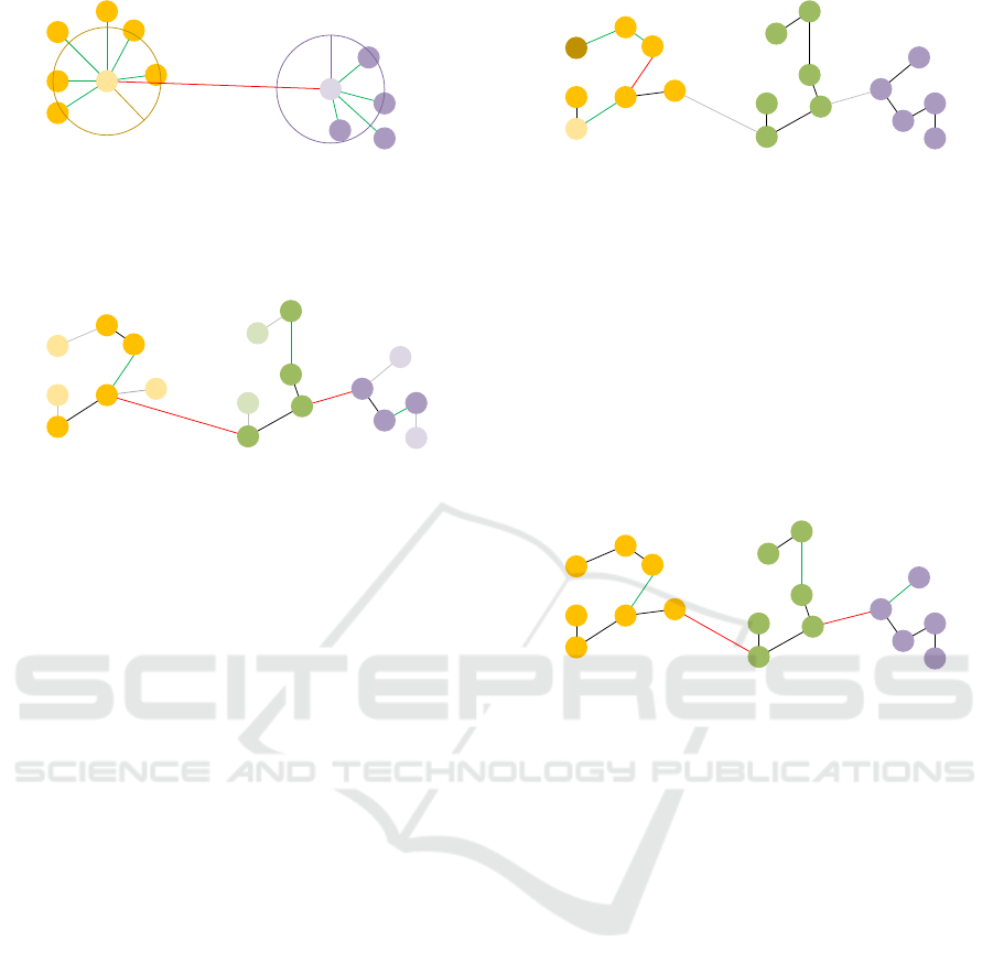
Figure 4: An example for the MRD between the light yel-

low and the light purple object. The circles around the

object represent the core distance of each object based on

the (green) similarity to objects in the same cluster. As the

(red) distance between both objects is bigger, this distance

is dominating the MRD.

Figure 5: An example of the computation of the DBCV. The

Sparsity per cluster is depicted as the green edge in each

cluster. The light gray edges are not part of this computa-

tion, as they connect to border objects. The red edges rep-

resent the Separation between two clusters as the minimum

distance between objects of these. The lighter coloured ob-

jects are excluded as those are border objects.

step of this algorithm is to adjust the distance between

two objects by ﬁrst assigning a core distance to each

object based on the density of other objects of the

same cluster and secondly replacing the “normal” dis-

tance between two objects by the maximum of each

objects core distance and the “normal” distance be-

tween those objects as Mutual Reachability Distance

(MRD). As the core distance will be high for an object

in a sparse region, this will raise the distance between

objects in sparse regions, whereas it will have little

effect in dense regions or for objects far apart. An

example of this computation can be seen in Figure 4.

Using this MRD, an MST is build in each cluster,

which is then pruned of its border object, which are

only connected by a single edge. Now, the DBCV for

each cluster is based on the Sparsity, the maximum

edge of these MSTs and the Separation, which is the

minimum distance of a non-border object to any non-

border object of a different cluster. An example of this

can be seen in Figure 5. To combine these, the Spar-

sity is deducted from the Separation and the result is

normalized by the bigger of these numbers. The result

for the complete clustering is the weighted average of

each cluster.

3.2.2 IC-av

Intracluster average gap (IC-av) (Bay

a and Granitto,

2013) is an approach penalizing clusterings with long

distances on the shortest path on an MST between

Figure 6: An example for the calculation for the path dis-

tance for IC-av of the light yellow and the dark yellow point.

The green and red edges comprise the path between those

objects. The red edge is used as distance between the ob-

jects, as it is the longest edge on the path. The weight of the

green edges is shorter, so those are not taken into account

for this distance.

two objects in the same cluster. The distance between

two objects is measured as the longest distance on the

shortest path between them. These distances are aver-

aged to get the IC-av.

3.2.3 DCVI

Figure 7: An example of the computation of the DCVI. The

Compactness resembles the green edges, whilst the Separa-

tion resembles the red edges.

Density-core-based clustering validation index

(DCVI) (Xie et al., 2020) is a similar measure to the

DBCV, but without using a sophisticated reachability

distance. The Separation of a cluster is measured as

the minimal distance of an object in the cluster to an

element in another cluster, whilst the Compactness

is measured as the maximum edge weight in the

MST of a cluster. The Compactness is divided by

the Separation to gain each clusters value, which is

averaged over all clusters.

3.2.4 CVDD

Another Approach is the Cluster Validity index

based on Density-involved Distance (CVDD) (Hu and

Zhong, 2019). Here, a density is generated based on

the k-nearest Neighbors of an object and a density-

connectivity distance is used. As this approach uses

a wide variety of correcting factors deduced from the

dataset, it is not possible for us to give more than the

crudest intuition of this method in our given space, so

we refer to the original paper for more information.

DATA 2025 - 14th International Conference on Data Science, Technology and Applications

366

Figure 8: The Separation of the light yellow objects re-

sembles the share of other clusters objects in its k nearest

Neighbors, whilst for the compactness, every distances two

objects in the same cluster (blue) are computed.

Figure 9: The local density of the light yellow objects for

the CDR is its closest distance to another object of the same

cluster, depicted by the green edge.

3.3 Other Methods

We use this umbrella subsection, to introduce a few

other, unique CVI, which do not use MSTs to approx-

imate the shape of the data.

3.3.1 CVNN

The Clustering validation index based on nearest

neighbours (CVNN) (Liu et al., 2013) uses Near-

est Neighbors for its notion of Separation, where the

maximum Separation of a cluster is the average num-

ber of other clusters elements in the k-Nearest Neigh-

bors of the clusters objects. The maximum Separation

of any cluster is used as Separation for the clustering.

The Compactness is measured as the average pairwise

distance between two objects of the same cluster. An

example for an object with k := 5 can be seen in Fig-

ure 8. In the end, Separation and Compactness of the

clustering are added to retrieve the value. A slight

variation of the weighting is found in (Halkidi et al.,

2015), which we also investigate as CVNN hal.

3.3.2 CDR

Another CVI is the Contiguous Density Region

(CDR) index (Rojas Thomas and Santos Pe

nas,

2021). In this CVI, the local density is measured by

the distance to the next object in the same cluster. The

notion of the CDR is, that this local density should be

very close the average density of the same cluster.

3.3.3 VIASCKDE

The Validity Index for Arbitrary-Shaped Clusters

Based on the Kernel Density Estimation (VI-

Figure 10: Exemplary VIASCKDE computation of the light

yellow element. The (blue) distances between the light yel-

low element and the other yellow elements are used to com-

pute the Compactness, while the (red) distances to the ele-

ments of the green cluster are used for the Separation. The

elements of the purple cluster are not used for this Silhou-

ette. The purple lines represent the isolines of the KDE, so

that elements inside those lines will have a higher weight.

Frequency

Distance

Figure 11: An illustration of the DSI computation. The

(green) distances of the light yellow object to the other yel-

low objects are part of the inner cluster distances of the yel-

low cluster. The (red) distances to objects of the other clus-

ters are part of the between cluster distances of the yellow

cluster. The difference between these histograms (seen on

the right) is used to calculate the DSI for the cluster.

ASCKDE) (S¸ enol, 2022) is very similar to the SWC

(see subsubsection 3.1.1). However, each object is

valued by the weight of a Kernel Density Estimation

of the dataset, meaning objects in more populated re-

gions will have a higher weight.

3.3.4 DSI

In the Distance-based Separability Index (DSI) (Guan

and Loew, 2022), the distances inside one cluster are

compared to the distances to objects of other clusters.

Instead of directly using the distances in the computa-

tions, two sets of distances are generated, comprising

the inner-cluster and the between-cluster distances of

one cluster. Then the difference between those his-

tograms is computed to gain a value for this cluster.

These values get averaged to retrieve a value for the

complete cluster.

3.4 Used Distances

The notion of similarity used to compute the dis-

tance between two objects plays an important role

in the evaluation of a clustering. Almost all pre-

sented methods are able to cope with different dis-

tance metrics without any problem. The exception

are the VRC, which directly works on the vector rep-

resentation of the objects, the S Dbw, which needs a

Arbitrary Shaped Clustering Validation on the Test Bench

367

Figure 12: An illustration of the DC-distance computation

between the blue and the green object. The edges depict the

MST of the dataset. The gray edges are ignored, because

they are not part of the path between both objects. The black

edges are shorter than the red edge, which resembles the

distance between both objects.

midpoint of clusters and between two objects and the

VIASCKDE, which needs a KDE based on the dis-

tance between objects. We will investigate all other

methods not only using the Euclidean distance, but

also the DC-distance (Beer et al., 2023). The DC-

distance measures the distance between two objects

in a density-connectivity based fashion, so that us-

ing this distance function even classical CVI like the

SWC should be able to ﬁnd arbitrary shaped cluster-

ings. Similar to the DBCV, every object is assigned

a core distance, which is the distance to its µ nearest

neighbor. It also uses a mutual reachability distance,

where the MRD between two objects is the maximum

of both objects core distance and their Euclidean dis-

tance. To ﬁnd the DC-distance between two objects,

an MST is build on the dataset using the MRDs. The

distance is now the longest edge on the path between

two points on this MST.

4 EXPERIMENTS

In this section, we will describe our experiments.

will start with a description of the used datasets (sub-

section 4.1), before we will explain which algorithms

were used to generate clusterings (subsection 4.2). To

conclude this section, we will describe the setup used

to generate our results (subsection 4.3).

4.1 Datasets

In order to generate valuable and qualitative results,

we generate datasets using the Densired dataset gen-

erator (Jahn et al., 2024). This generator is capable of

generating clusterings of arbitrary shapes, which are

guaranteed to be density-connectivity separable and

allows for a variety of parameters to be tuned. In addi-

tion to the parameters discussed in the following para-

graphs, we set the parameters safety to False, which

allows noise points to be generated next to or inside

a cluster. For each parameterization, we created three

Our implementation of the CVI can be found under

https://github.com/g-schlake/ASCVI

datasets to prevent an inﬂuence of chance and to see

the variance of the CVI in similar datasets. The actual

values used for each test can be seen in Table 1.

Dimensionality. The ﬁrst metafeature we tuned was

the dimensionality. It is wide known, that real datasets

can contain many dimensions. However, many ar-

bitrary shaped, synthetical datasets are only two- or

three-dimensional, so many evaluations of methods or

even surveys like (Schlake and Beecks, 2024b) might

be misled, if CVI perform especially well in the lower

dimensional space. We used 5 dimensions as standard

value in order to not prevent former mistakes of only

investigating a low dimensional space, but also to not

investigate too high dimensional spaces.

Number of Clusters. The number of clusters is an-

other interesting metafeature of datasets. While some

algorithms take information of all clusters into ac-

count, others only compare neighboring clusters. We

change the number of clusters in the clustering to see,

whether this leads to CVI scaling with the number of

clusters. Our default will be 10 clusters.

Overlap Factor. Overlaps between clusters have

been shown to be a problem for a number of density-

connectivity based CVI (Schlake and Beecks, 2024b).

In the generation of datasets, the separability between

two clusters is guaranteed based on the Overlap fac-

tor. By lowering this value below 1, overlaps between

two clusters can happen, which can lead to problems

for some CVI. Our standard value will be 1.1, to en-

sure no overlaps for our standard tests.

Number of Connections. Another way to generate

overlapping clusters is the existence of lower density

bridges between two clusters. With this parameter,

we can control, how many low linkage bridges exist

between different clusterings. As standard, we will

have no bridges between two clusters.

Noise Ration. Another very important factor is the

ability to handle noise. While noise is occurring in

almost all real world scenarios, many CVI are not able

to handle it properly. For this reason, our standard

noise ratio will be 0.

Number of Objects. Our last tests will be about the

number of objects. As datasets tend to vary in size,

we will use datasets in varying sizes. Our standard

datasets will have the size of 5.000.

DATA 2025 - 14th International Conference on Data Science, Technology and Applications

368

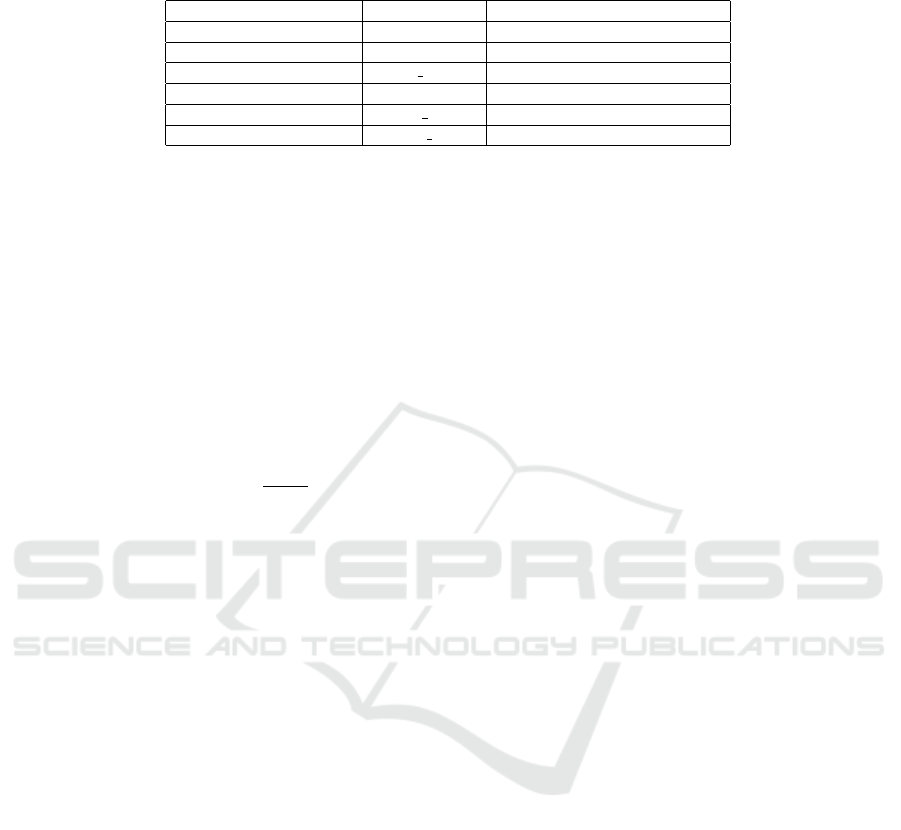
Table 1: The different metafeatures, their respective parameters and the investigated values. The default value is printed in

bold.

Metafeature Parameter Values

Dimensionality dim 2, 3, 5, 10, 20

Number of Clusters clunum 2, 3, 5, 10, 20

Overlap Factor min dist 0.5, 0.8, 0.9, 1, 1.1, 1.2, 1.3

Number of Connections connections 0, 1, 4, 8, 10

Noise Ration ratio noise 0, 0.05, 0.1, 0.2

Number of Objects data num 100, 500, 1.000, 5.000, 10.000

4.2 Used Algorithms

To generate a number of clusterings, we use three

different clustering algorithms, out of which one is

partition-based and two are density-based.

The kMeans (McQueen, 1967) algorithm is a very

wide known algorithm to assign clusters based on

centroids. This algorithm is not capable of ﬁnding

arbitrary shaped clusters, but it is important to also in-

clude a partition based algorithm, as otherwise a lack

of partition based results might lead to CVI choosing

density based results, because they lack higher valued

partition based alternatives. For the k Parameter, we

used the values ranging between

clunum

and 3· clunum

and the implementation from (Pedregosa et al., 2011),

so we had (mostly) 27 different values.

DBSCAN (Ester et al., 1996) is a widely known

algorithm for density-connectivity based clustering,

which is still in wide use today (Schubert et al., 2017).

In this algorithm, objects with enough other objects in

close proximity are regarded as core objects of a clus-

ter and objects, which are close to these are part of the

same cluster. We used the implementation from (Pe-

dregosa et al., 2011), where we set MinPts to the even

values in [4,20] and eps to 100 equidistant values

in the distances between the minimum and the max-

imum distance between two objects, resulting in the-

oretically up to 900 clusterings. However, as most

of these are identical due to the very minor changes,

only the differing ones (maximum 102 per Dataset)

are considered.

An updated approach is HDBSCAN (Campello

et al., 2015), which uses hierarchical properties to

make a decision for a data scientist easier. We used

the implementation in (McInnes et al., 2017), where

we only tuned the MinPts parameter, which we set to

the even values in [4,20], resulting in 8 clusterings per

dataset.

4.3 Experimental Setup

In order to evaluate our clusterings, we test how well

they select a clustering resembling the ground truth

of the dataset. Even though the clustering Problem

in general is ambiguous (von Luxburg et al., 2012),

we can assume that the ground truth of our generated

datasets is what we are looking for, as it was generated

and evaluated with the same notion of similarity and

“good” clusterings. For every test, we have generated

3 datasets for each test value, which are then clus-

tered using our three algorithms using the described

parameters. Following this, we select the best cluster

on each dataset for each CVI based on the value of the

CVI. As not every CVI can process noise objects, we

remove objects clustered as noise from the clustering

and multiply the result of the clustering with a penalty

term based on the share of noise in the dataset like de-

scribed in (Schlake and Beecks, 2024b). Where pos-

sible, we also evaluated the clusterings using the DC-

distance as distance function. As we have 3 datasets

per test and value, we get 3 results per test, value

and CVI, out of which we will mostly focus on the

median. We will evaluate the quality of each clus-

tering by measuring the Adjusted Mutual Information

(AMI) (Nguyen et al., 2009) with the ground truth.

As the AMI has no special considerations for noise,

we will assign every noise object to its own, singleton

cluster. This will prevent the AMI from confusing a

cluster in one clustering with similar noise objects in

the other clustering.

5 RESULTS

In the following section, we will present the results of

our 6 tests. Every subsection will show the results of

both used distances. We will start with the dimension-

ality (subsection 5.1) and number of clusters (subsec-

tion 5.2), before we will have a look at the overlap

factor (subsection 5.3) and the number of connections

(subsection 5.4). We will ﬁnish with the noise ratio

(subsection 5.5) and the number of objects (subsec-

tion 5.6).

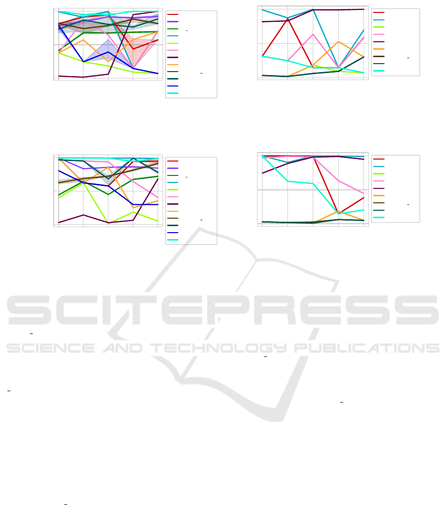
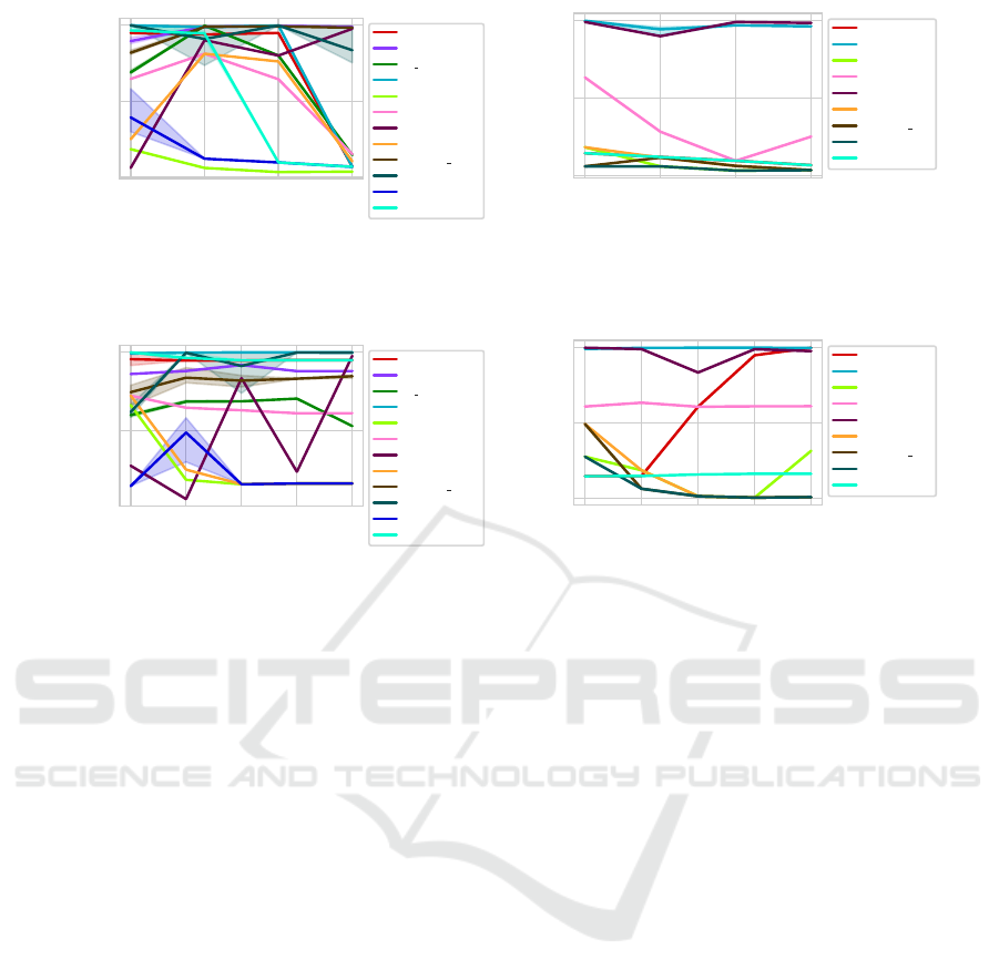
5.1 Dimensionality

When looking at the results at different dimensional-

ities, we see widely varying results in many datasets

Arbitrary Shaped Clustering Validation on the Test Bench

369

2 3 5 10 20

Number of dimensions

0.0

0.5

1.0

AMI

SWC

VRC

S Dbw

DBCV

IC-av

DCVI

CVDD

CVNN

CVNN hal

CDR

VIASCKDE

DSI

(a) Euclidean.

2 3 5 10 20

Number of dimensions

0.0

0.5

1.0

AMI

SWC

DBCV

IC-av

DCVI

CVDD

CVNN

CVNN hal

CDR

DSI

(b) DC-distance.

Figure 13: AMI per CVI using datasets of different dimensionalities. The thick line represents the median value on three

datasets, while the shaded area is based on maximum and minimum value.

2 3 5 10 20

Number of clusters

0.0

0.5

1.0

AMI

SWC

VRC

S Dbw

DBCV

IC-av

DCVI

CVDD

CVNN

CVNN hal

CDR

VIASCKDE

DSI

(a) Euclidean.

2 3 5 10 20

Number of clusters

0.0

0.5

1.0

AMI

SWC

DBCV

IC-av

DCVI

CVDD

CVNN

CVNN hal

CDR

DSI

(b) DC-distance.

Figure 14: AMI per CVI using datasets with a different number of clusters. The thick line represents the median value on

three datasets, while the shaded area is based on maximum and minimum value.

(see Figure 13). When focusing on the Euclidean dis-

tance (Figure 13a), it can be seen that DSI, VRC,

CVNN hal and CDR seem to ﬁnd good clusterings

using all dimensionalities. IC-av and VIASCKDE

struggle to evaluate the clusterings correctly in higher

dimensional spaces. CVNN and DCVI have high

variations between the different dimensionalities. The

S Dbw struggles in the two-dimensional case, but is

constant in all the other dimensionalities. The SWC

and the DBCV seem to deliver good results, but both

have a negative outlier at 10 dimensions. It can be

seen, that VIASCKDE, DCVI, SWC and CDR have

different results for the different datasets and are quite

sensitive to minimal changes.

When looking at the results using the DC-distance

(Figure 13b), it can be seen that the CVDD delivers

good results using all dimensionalities, whilst IC-av,

CVNN, CVNN hal, DSI and have struggles to ﬁnd

good clusterings. SWC, DBCV and DCVI have vary-

ing results.

5.2 Number of Clusters

When looking at the varying number of clusters us-

ing the Euclidean distance (Figure 14a), it can be seen

that DBCV, DSI and produce good clusterings regard-

less of the number of clusters. CVNN, VIASCKDE

and IC-av work well for 2 and 3 clusters, but strug-

gle to ﬁnd good clusterings using more clusters. The

SWC works well only for a high number of clus-

ters. Similarly, the CVDD has low results on the most

numbers of clusters but works well using 20 clusters.

CVNN hal seems to ﬁnd better clusterings, the more

clusters are in the ground truth.

Using the DC-dist, most algorithms seem to ei-

ther ﬁnd very good (SWC, DCVI, DBCV, CVDD) or

very bad (CVNN, CVNN hal, CDR, IC-av) cluster-

ings with 5 or less clusters. The exception is DSI,

which only ﬁngds good clusterings with 2 clusters and

struggles even from 3 on. The SWC and DCVI strug-

gle, when there are more than 5 clusters present.

5.3 Overlap Factor

The only notable change in the CVI using the Overlap

happens between 0.8 and 0.9. DBCV, DCVI, SWC

and CDR produce much better results when there are

no overlaps. CVDD, CVNN and IC-av produce their

only good results if there are overlaps.

The trend is similar using the DC-distance. How-

ever, the SWC and CDR are producing better results

with overlaps using this distance.

DATA 2025 - 14th International Conference on Data Science, Technology and Applications

370

0.5 0.8 0.9 1 1.1 1.2 1.3

Overlap factor

0.5

1.0

AMI

SWC

VRC

S Dbw

DBCV

IC-av

DCVI

CVDD

CVNN

CVNN hal

CDR

VIASCKDE

DSI

(a) Euclidean.

0.5 0.8 0.9 1 1.1 1.2 1.3

Overlap factor

0.5

1.0

AMI

SWC

DBCV

IC-av

DCVI

CVDD

CVNN

CVNN hal

CDR

DSI

(b) DC-distance.

Figure 15: AMI per CVI using datasets with different overlap factors. The thick line represents the median value on three

datasets, while the shaded area is based on maximum and minimum value.

0 1 4 8 10

Number of connections between clusters

0.0

0.5

1.0

AMI

SWC

VRC

S Dbw

DBCV

IC-av

DCVI

CVDD

CVNN

CVNN hal

CDR

VIASCKDE

DSI

(a) Euclidean.

0 1 4 8 10

Number of connections between clusters

0.0

0.5

1.0

AMI

SWC

DBCV

IC-av

DCVI

CVDD

CVNN

CVNN hal

CDR

DSI

(b) DC-distance.

Figure 16: AMI per CVI using datasets with a different number of connections. The thick line represents the median value on

three datasets, while the shaded area is based on maximum and minimum value.

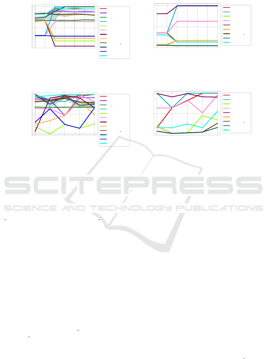
5.4 Number of Connections

When looking at the presence of connections between

different clusters using the Euclidean distance (Fig-

ure 16b), it can be seen that this has little effect on

S Dbw, DBCV, DSI, SWC and CVNN hal. How-

ever, more connections seem to lead to better results

for CVDD, CVNN and VIASCKDE. VRC and DCVI

have no general trend, but a relatively large drop at 4

connections.

Using the DC-distance (Figure 16a), you can see

that the effect of the number of connections is much

smaller. SWC, DCVI, DSI and IC-av have slight trend

to ﬁnd better clusterings with a higher number of con-

nections between clusters. Apart from this, most CVI

have a stable trend with little outliers.

5.5 Noise Ratio

When looking at the noise ratio using the Euclidean

distance (Figure 17a), it can be seen that most algo-

rithms (all apart from IC-av, S Dbw, CVDD, VRC

and CVNN hal) have a massive drop in selecting the

correct clustering when too many outliers are present.

This drop happens earlier for the DSI than for the

other methods.

Using the DC-distance (Figure 17b), the noise ra-

tios chosen by us have little inﬂuence on the perfor-

mance of the CVI.

5.6 Number of Objects

When looking at the number of objects, you can see

that most CVI stay constant using the Euclidean dis-

tance (Figure 18a), IC-av and CVNN show much bet-

ter results using only a little number of object. The

performance of CVDD has a general positive trend,

but also has many negative outliers.

Using the DC-distance (Figure 14b), you can see

that the SWC works better, the more objects are

present.

6 DISCUSSION

In this section, we will discuss our results and con-

clude our ﬁndings. We have seen that some CVI like

CVDD work well in high dimensional cases or with

many clusters and might have struggles in “easier”

cases, which are similar to many well known bench-

mark datasets, explaining the poor results in previous

surveys (Schlake and Beecks, 2024b). Of all CVI, the

DBCV seems to work well in most scenarios, except

for a high number of outliers, where CVNN hal, CDR

and CVDD perform better. Interestingly, CVNN, IC-

av and CVDD perform better, when there are overlaps

Arbitrary Shaped Clustering Validation on the Test Bench

371

0 0.05 0.1 0.2

Noise ratio

0.0

0.5

1.0

AMI

SWC

VRC

S Dbw

DBCV

IC-av

DCVI

CVDD

CVNN

CVNN hal

CDR

VIASCKDE

DSI

(a) Euclidean.

0 0.05 0.1 0.2

Noise ratio

0.0

0.5

1.0

AMI

SWC

DBCV

IC-av

DCVI

CVDD

CVNN

CVNN hal

CDR

DSI

(b) DC-distance.

Figure 17: AMI per CVI using datasets with different noise ratios. The thick line represents the median value on three

datasets, while the shaded area is based on maximum and minimum value.

100 500 1000 5000 10000

Number of objects

0.5

1.0

AMI

SWC

VRC

S Dbw

DBCV

IC-av

DCVI

CVDD

CVNN

CVNN hal

CDR

VIASCKDE

DSI

(a) Euclidean.

100 500 1000 5000 10000

Number of objects

0.0

0.5

1.0

AMI

SWC

DBCV

IC-av

DCVI

CVDD

CVNN

CVNN hal

CDR

DSI

(b) DC-distance.

Figure 18: AMI per CVI using datasets of different sizes. The thick line represents the median value on three datasets, while

the shaded area is based on maximum and minimum value.

between clusters. This might be interesting for further

research. We also ﬁgured out that the combination

of DC-distance and DBCV or CVDD will aptly ﬁnd

clusterings in all our scenarios.

However, our results have to be treated with some

caveats. While we did investigate all these different

factors in isolation, the combination of these factors

might lead to completely different results. An inves-

tigation of all combinations of these properties is not

possible due to their sheer numbers. The second big

caveat is that the quality of these results is depen-

dent on the quality of the Densired dataset generator.

While many CVI have trends, which are expected or

invariant and support the use of this dataset generator,

some results are unexpected and unintuitive. Obvi-

ously, this might be due to an interesting behaviour

of the corresponding CVI, but also some subopti-

mal generated datasets are possible. Another caveat

is, that there is no possibility to measure the “arbi-

trary” of a clusterings shape. It is possible that some

datasets actually contain partitioning based clusters,

which would explain the good performance of the

SWC. However, this unintuitively good performance

matches the results of (Schlake and Beecks, 2024b),

so that it could be, that there are some properties mak-

ing the SWC better suited for arbitrary shaped data

than known.

REFERENCES

Ankerst, M., Breunig, M. M., Kriegel, H., and Sander, J.

(1999). OPTICS: ordering points to identify the clus-

tering structure. In SIGMOD Conference, pages 49–

60. ACM Press.

Bay

a, A. E. and Granitto, P. M. (2013). How many clus-

ters: A validation index for arbitrary-shaped clus-

ters. IEEE ACM Trans. Comput. Biol. Bioinform.,

10(2):401–414.

Beecks, C., Uysal, M. S., and Seidl, T. (2010). Signature

quadratic form distance. In CIVR, pages 438–445.

ACM.

Beer, A., Draganov, A., Hohma, E., Jahn, P., Frey, C.

M. M., and Assent, I. (2023). Connecting the dots -

density-connectivity distance uniﬁes dbscan, k-center

and spectral clustering. In KDD, pages 80–92. ACM.

Berndt, D. J. and Clifford, J. (1994). Using dynamic time

warping to ﬁnd patterns in time series. In KDD Work-

shop, pages 359–370.

Cali

nski, T. and Harabasz, J. (1974). A dendrite method

for cluster analysis. Commun. Stat. - Theory Methods,

3(1):1–27.

Campello, R. J. G. B., Moulavi, D., Zimek, A., and Sander,

J. (2015). Hierarchical density estimates for data

clustering, visualization, and outlier detection. ACM

Trans. Knowl. Discov. Data, 10(1):5:1–5:51.

Deborah, L. J., Baskaran, R., and Kannan, A. (2010). A sur-

vey on internal validity measure for cluster validation.

IJCSES, 1(2):85–102.

DATA 2025 - 14th International Conference on Data Science, Technology and Applications

372

Ester, M., Kriegel, H., Sander, J., and Xu, X. (1996). A

density-based algorithm for discovering clusters in

large spatial databases with noise. In KDD, pages

226–231. AAAI Press.

Gan, J. and Tao, Y. (2015). DBSCAN revisited: Mis-claim,

un-ﬁxability, and approximation. In SIGMOD Con-

ference, pages 519–530. ACM.

Guan, S. and Loew, M. H. (2022). A distance-based sepa-

rability measure for internal cluster validation. Int. J.

Artif. Intell. Tools, 31(7):2260005:1–2260005:23.

Halkidi, M., Batistakis, Y., and Vazirgiannis, M. (2001). On

clustering validation techniques. J. Intell. Inf. Syst.,

17:107–145.

Halkidi, M. and Vazirgiannis, M. (2001). Clustering valid-

ity assessment: Finding the optimal partitioning of a

data set. In ICDM, pages 187–194. IEEE Computer

Society.

Halkidi, M., Vazirgiannis, M., and Hennig, C. (2015).

Method-independent indices for cluster validation and

estimating the number of clusters. In Handbook

of cluster analysis, pages 616–639. Chapman and

Hall/CRC.

Hassan, B. A., Tayfor, N. B., Hassan, A. A., Ahmed, A. M.,

Rashid, T. A., and Abdalla, N. N. (2024). From a-to-z

review of clustering validation indices. Neurocomput-

ing, 601:128198.

Hu, L. and Zhong, C. (2019). An internal validity index

based on density-involved distance. IEEE Access,

7:40038–40051.

Jahn, P., Frey, C. M. M., Beer, A., Leiber, C., and Seidl, T.

(2024). Data with density-based clusters: A generator

for systematic evaluation of clustering algorithms. In

ECML/PKDD (7), volume 14947 of Lecture Notes in

Computer Science, pages 3–21. Springer.

Kaufman, L. and Rousseeuw, P. J. (1990). Partitioning

Around Medoids (Program PAM), chapter 2, pages

68–125. John Wiley & Sons, Ltd.

Li, W. and Zhou, Z. (2023). Ac: A data generator for eval-

uation of clustering. Authorea Preprints.

Lim, A., Rodrigues, B., Wang, F., and Xu, Z. (2005). k-

center problems with minimum coverage. Theo. Com-

put. Sci., 332(1-3):1–17.

Liu, Y., Li, Z., Xiong, H., Gao, X., Wu, J., and Wu, S.

(2013). Understanding and enhancement of internal

clustering validation measures. IEEE Trans. Cybern.,

43(3):982–994.

McInnes, L., Healy, J., and Astels, S. (2017). hdbscan: Hi-

erarchical density based clustering. J. Open Source

Softw., 2(11):205.

McQueen, J. (1967). Some methods for classiﬁcation and

analysis of multivariate observations. In Proc. Fifth

Berkeley Symposium on Mathematical Statistics and

Probability, 1967, pages 281–297.

Moulavi, D., Jaskowiak, P. A., Campello, R. J. G. B.,

Zimek, A., and Sander, J. (2014). Density-based clus-

tering validation. In SDM, pages 839–847. SIAM.

Nguyen, X. V., Epps, J., and Bailey, J. (2009). Informa-

tion theoretic measures for clusterings comparison: is

a correction for chance necessary? In ICML, volume

382 of ACM International Conference Proceeding Se-

ries, pages 1073–1080. ACM.

Parsons, L., Haque, E., and Liu, H. (2004). Subspace clus-

tering for high dimensional data: a review. SIGKDD

Explor., 6(1):90–105.

Pedregosa, F., Varoquaux, G., Gramfort, A., Michel, V.,

Thirion, B., Grisel, O., Blondel, M., Prettenhofer, P.,

Weiss, R., Dubourg, V., VanderPlas, J., Passos, A.,

Cournapeau, D., Brucher, M., Perrot, M., and Duch-

esnay, E. (2011). Scikit-learn: Machine learning in

python. J. Mach. Learn. Res., 12:2825–2830.

Rojas Thomas, J. C. and Santos Pe

nas, M. (2021). New

internal clustering validation measure for contigu-

ous arbitrary-shape clusters. Int. J. Intell. Syst.,

36(10):5506–5529.

Rousseeuw, P. J. (1987). Silhouettes: a graphical aid to

the interpretation and validation of cluster analysis. J.

Comput. Appl. Math., 20:53–65.

Ruspini, E. H., Bezdek, J. C., and Keller, J. M. (2019).

Fuzzy clustering: A historical perspective. IEEE

Comput. Intell. Mag., 14(1):45–55.

Schlake, G. S. and Beecks, C. (2023). Towards automated

clustering. In IEEE Big Data, pages 6268–6270.

IEEE.

Schlake, G. S. and Beecks, C. (2024a). The skyline operator

to ﬁnd the needle in the haystack for automated clus-

tering. In IEEE Big Data, pages 6117–6122. [IEEE.

Schlake, G. S. and Beecks, C. (2024b). Validating arbi-

trary shaped clusters - A survey. In DSAA, pages 1–12.

IEEE.

Schlake, G. S., Pernklau, M., and Beecks, C. (2024). Au-

tomated exploratory clustering. In IEEE Big Data,

pages 5711–5720. IEEE.

Schubert, E., Sander, J., Ester, M., Kriegel, H. P., and Xu, X.

(2017). DBSCAN revisited, revisited: why and how

you should (still) use DBSCAN. TODS, 42(3):1–21.

S¸enol, A. (2022). VIASCKDE index: A novel internal clus-

ter validity index for arbitrary-shaped clusters based

on the kernel density estimation. Comput. Intell. Neu-

rosci., 2022.1:4059302.

von Luxburg, U., Williamson, R. C., and Guyon, I. (2012).

Clustering: Science or art? In ICML Unsupervised

and Transfer Learning, volume 27 of JMLR Proceed-

ings, pages 65–80. JMLR.org.

Ward Jr, J. H. (1963). Hierarchical grouping to optimize an

objective function. JASA, 58(301):236–244.

Xie, J., Xiong, Z., Dai, Q., Wang, X., and Zhang, Y. (2020).

A new internal index based on density core for clus-

tering validation. Inf. Sci., 506:346–365.

Arbitrary Shaped Clustering Validation on the Test Bench

373