Knapsack and Shortest Path Problems Generalizations from a

Quantum-Inspired Tensor Network Perspective

Sergio Mu

niz Subi

nas

1 a

, Jorge Mart

ınez Mart

ın

1 b

, Alejandro Mata Ali

1 c

, Javier Sedano

1 d

and

Angel Miguel Garc

ıa-Vico

2 e

Instituto Tecnol

ogico de Castilla y Le

on, Burgos, Spain

Andalusian Research Institute in Data Science and Computational Intelligence (DaSCI), University of Ja

en,

23071 Ja

en, Spain

Keywords:

Quantum Computing, Tensor Networks, Combinatorial Optimization, Quantum-Inspired.

Abstract:

In this paper, we present two tensor network quantum-inspired algorithms to solve the knapsack and the short-

est path problems, and enables to solve some of its variations. These methods provide an exact equation which

returns the optimal solution of the problems. As in other tensor network algorithms for combinatorial opti-

mization problems, the method is based on imaginary time evolution and the implementation of restrictions

in the tensor network. In addition, we introduce the use of symmetries and the reutilization of intermediate

calculations, reducing the computational complexity for both problems. To show the efﬁciency of our imple-

mentations, we carry out some performance experiments and compare the results with those obtained by other

classical algorithms.

1 INTRODUCTION

Combinatorial optimization has become a wide ﬁeld

of study due to the large number of industrial and

academic applications in different disciplines, for

instance, engineering or logistics. Some of the

most prominent and extensively studied problems are

route optimization (traveling salesman problem (La-

porte, 1992; Korte and Vygen, 2008) or the short-

est path (Dijkstra, 1959; Hart et al., 1968)), task

scheduling (job-shop scheduling problem (Lenstra,

1992; Dauz

ere-P

es et al., 2024)) and constrained

optimization (knapsack (Mathews, 1896; Bateni et al.,

2018) or bin packing (Korte and Vygen, 2000; Egor

et al., 2022)). The fact that most of these problems

are NP-hard makes exact resolution methods compu-

tationally unaffordable. With the objective of solv-

ing these problems, it is common to draw upon ap-

proximations, generally obtaining a suboptimal re-

sult. However, in many industrial cases, the focus

is on ﬁnding a solution that works well enough in a

https://orcid.org/0009-0008-7590-0149

https://orcid.org/0009-0004-9336-3165

https://orcid.org/0009-0006-7289-8827

https://orcid.org/0000-0002-4191-8438

https://orcid.org/0000-0003-1583-2128

reasonable time, rather than looking for the best pos-

sible outcome. Some of the most used classical ap-

proximation techniques are greedy approaches (Gutin

and Yeo, 2007), reinforcement learning (Wang and

Dong, 2024), genetic algorithms (Pilcher, 2023) or

simulated annealing (Katangur et al., 2002).

Meanwhile, due to the development of quantum

technologies, new ways of approaching combinatorial

optimization problems have been proposed. Among

other applications, it is possible to address the solu-

tion for quadratic unconstrained binary optimization

(QUBO) (Glover et al., 2019) problems with quan-

tum algorithms such as the quantum approximate op-

timization algorithm (QAOA) (Farhi et al., 2014) or

the variational quantum eigensolver (VQE) (Peruzzo

et al., 2014). Likewise, Constrained Quadratic Mod-

els (CQM) and Binary Quadratic Models (BQM) can

be solved with quantum annealers (Benson et al.,

2023). With the current status of quantum com-

puters hardware, where qubits are noisy and unreli-

able, no improvement in the state-of-the-art has been

achieved. Nevertheless, due to the strong theoret-

ical basis of these algorithms, researchers have de-

veloped quantum-inspired strategies, with tensor net-

works (TN) emerging as one of the most populars (Bi-

amonte and Bergholm, 2017; Biamonte, 2020). This

discipline consists in taking advantage of some prop-

Subiñas, S. M., Martín, J. M., Ali, A. M., Sedano, J. and García-Vico, Á. M.

Knapsack and Shortest Path Problems Generalizations from a Quantum-Inspired Tensor Network Perspective.

DOI: 10.5220/0013489000004525

In Proceedings of the 1st International Conference on Quantum Software (IQSOFT 2025), pages 81-88

ISBN: 978-989-758-761-0

erties of tensor algebra to compress information or

perform calculations in a more efﬁcient way. More-

over, by applying tensor decomposition operations

such as singular value decomposition (SVD) (Golub

and Kahan, 1965) in a truncated way, it is possible to

make approximations losing the least relevant infor-

mation. Numerous studies show the computational

advantages of tensor networks in a wide variety of

applications, for instance, in the simulation of quan-

tum systems (Biamonte, 2020), compression of neu-

ronal networks (Qing et al., 2024), anomaly detec-

tion (Wang et al., 2020; Ali et al., 2024a) or com-

binatorial optimization problems (Hao et al., 2022),

which are the object of study of this paper.

In this paper, we present two tensor network algo-

rithms to solve the knapsack and shortest path prob-

lems. Our method is based on previous works applied

to traveling salesman problem (Ali et al., 2024b),

QUBO problems (Ali et al., 2024d) and task schedul-

ing (Ali et al., 2024c). The objective of this study is

to present an analytical methodology for solving com-

binatorial optimization problems, rather than a com-

putational advantage in such problems. Following

the results in (Ali, 2025), it provides an exact equa-

tion that returns the optimal solution to these prob-

lems. We compare the results of our implementations

against some classical algorithms.

2 KNAPSACK PROBLEM

Given a set of n different item classes, where the i-

th class can be selected up to c

times, each with

an associated weight w

∈ N and value v

∈ R

, the

knapsack problem consists in ﬁnding the conﬁgura-

tion ⃗x = (x

,..,x

n−1

) that maximizes

V (⃗x) =

n−1

∑

i=0

subject to W (⃗x) =

n−1

∑

i=0

≤ Q,

∈ [0,c

] ∀i ∈ [0,n − 1],

(1)

being x

the number of times the i-th class has been

selected, V (⃗x) the total value of the items, W (⃗x) the

total weight of the items in the knapsack and Q the

maximum weight capacity. There are different vari-

ants of this problem, the most popular being the 0-1

knapsack, where each class can be selected only once,

∈ {0,1}. These instances variants can be solved

exactly with a time complexity of O(nQ) and space

complexity O(nQ).

2.1 Tensor Network Algorithm

The idea of our algorithm is to take advantage of the

imaginary time evolution to generate a state whose

basis state with the greatest amplitude represents the

optimal conﬁguration. Due to the high number of

possible combinations, we cannot know the ampli-

tude of all combinations at once, and hence determine

the highest probability state. Therefore, we employ

a method that consists in determining each variable

separately, by projecting the state into each subspace

associated with the respective variable.

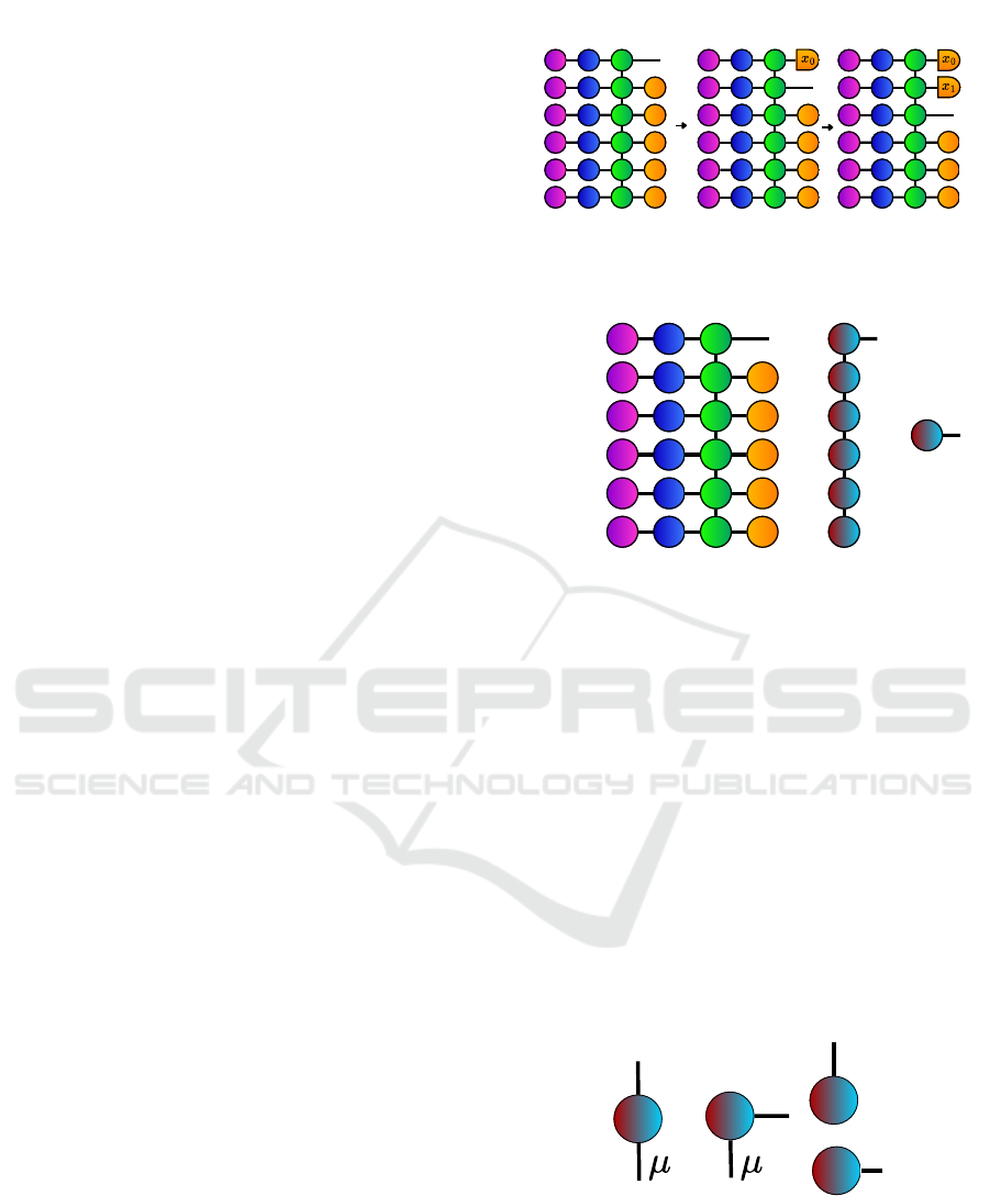
2.1.1 Quantum-Inspired Tensor Network

Our knapsack problem algorithm is based on ten-

sor algebra and some properties of quantum comput-

ing such as superposition or projected measurements.

Thus, we have developed a quantum-inspired tensor

network that incorporates the theoretical advantages

of quantum computing without being limited by its

constraints. The tensor network (see Fig. 2 a) can be

interpreted as a ‘quantum circuit’ that can be simu-

lated in four steps, each one corresponding to one of

the layers in the ﬁgure.

The system starts in a uniform superposition of n

variables, each one encoded in the basis states of a

qudit of dimension c

+ 1. This ﬁrst step corresponds

to the ﬁrst layer of tensors ‘+’ in Fig. 2 a, and the

mathematical representation of the resulting state is

|ψ

⟩ =

∑

⃗x

|⃗x⟩ =

n−1

i=0

∑

⟩. (2)

The next step consists of applying an imaginary time

evolution layer to the superposition that ampliﬁes the

basis states with a higher value. We implement this

with an operator S , which assigns to each state |⃗x⟩ an

exponential amplitude corresponding to its associated

value V (⃗x). The parameter τ scales the costs so that

the amplitudes differ exponentially from each other.

The state after applying this layer is

|ψ

⟩ =S|ψ

⟩ =

∑

⃗x

τV (⃗x)

|⃗x⟩. (3)

In order to eliminate incompatible conﬁgurations, we

apply a third layer that imposes the maximum capac-

ity constraint,

|ψ

⟩ = R (Q)|ψ

⟩ =

∑

⃗x

τV (⃗x)

R (Q)|⃗x⟩

R (Q)|⃗x⟩ = |⃗x⟩ if W (⃗x) ≤ Q,

(4)

where R (Q) is the operator that projects the state into

the subspace that fulﬁlls the maximum weight capac-

ity Q. This is implemented by a layer of R

tensors,

IQSOFT 2025 - 1st International Conference on Quantum Software

where the up index keeps track of the current weight

loaded at the knapsack until that qudit, while the down

index outputs the resultant weight after adding the

new qudit state. If this weight exceeds Q, the am-

plitude of the state is multiplied by zero.

Once obtained a system that has performed the

minimization and constraint, we need a method to ex-

tract the position of the largest element of the super-

position without checking all the possible combina-

tions. To do this, we have to take into account that,

for a sufﬁciently large τ, there will be a very high am-

plitude peak in the state of the optimal solution. In

order to achieve this, we apply a partial trace layer

to the tensor network except for the ﬁrst qudit. This

leads to the state

|ψ

⟩ =

∑

⃗z

⟨z

,...,z

n−1

|ψ

⟩ =

∑

⃗x|W (⃗x)≤Q

τV (⃗x)

⟩.

(5)

It can be interpreted as the resulting state from pro-

jecting |ψ

⟩ into the Hilbert space H

of the ﬁrst

qudit and it is equivalent as the quantum process of

measuring the ﬁrst qubit. The associated vector rep-

resentation is:

|ψ

⟩ =







⟨0 + · · · + |ψ

⟩

⟨1 + · · · + |ψ

⟩

⟨c

+ ··· + |ψ

⟩







, (6)

where each amplitude allows to determine the prob-

ability of |ψ

⟩ of being in their corresponding basis

states |x

⟩.

To determine the ﬁrst variable x

, we contract the

tensor network (see Fig. 2 a) to obtain |ψ

⟩, whose

highest amplitude value position corresponds to the

optimum value of the variable x

. To compute the

remaining variables, we use the same tensor network

but, instead of leaving free the index associated to the

ﬁrst variable, we free the index we want to obtain and

follow the same contraction process as in the previous

step. With this, we obtain the |ψ

⟩ state, from which

we determine the m-th variable. In each step, at the

end of the line of the variables that we have already

determined, we put a vector where all its elements are

zero, except the element corresponding to the chosen

value of the variable. This process is shown in Fig. 1.

2.1.2 Tensor Network Layout

Since it is possible to compress the information of the

four layers into a single layer in a convenient way, we

propose a direct implementation of the tensor network

in a chain structure (see Fig. 2). We deﬁne the tensors

following the index convention of Fig. 3.

a) b) c)

S⁰

S¹

S²

S³

S⁴

S⁵

R¹

R²

R³

R⁴

R⁵

S⁰

S¹

S²

S³

S⁴

S⁵

R⁰

R¹

R²

R³

R⁴

R⁵

S⁰

S¹

S²

S³

S⁴

S⁵

R⁰

R¹

R²

R³

R⁴

R⁵

Figure 1: Graphic representation of the iterative method of

the tensor network to obtain each variable.

S⁰

S¹

S²

S³

S⁴

S⁵

R⁰

R¹

R²

R³

R⁴

R⁵

M⁰

K¹

K²

K³

K⁴

K⁵

x₀

x₁

x₂

x₃

x₄

x₅

P⁰

a) b)

Figure 2: Tensor network solving the knapsack problem. a)

Tensor network solving the knapsack problem composed of

four column layers. From left to right: superposition (‘+’),

evolution (S), constraint (R) and tracing (‘+’). b) Com-

pressed version into a linear TN that implements all four

layers simultaneously. c) Contracted tensor.

From the ﬁgure, we can see that there are three

different types of tensors. The tensor M

, with ele-

ments M

iµ

, is associated with the ﬁrst qudit we want

to measure. This tensor is the result of the contrac-

tion between the superposition node ‘+’, the evolu-

tion node S

and the projector node R

. It outputs in-

formation about the state of the qudit throughout the

index i, and outputs the weight of the knapsack after

adding the new items throughout the index µ. There-

fore, the dimensions of the indexes i and µ are c

′

and

′

respectively, being Q

′

= Q + 1 and c

′

= c

+ 1 to

streamline the notation. The non-zero elements of the

b) c)

Figure 3: Nomenclature of the indexes of each tensor from

the tensor chain, where i corresponds to a variable index and

µ to a dependent index. a) A tensor from the middle of the

tensor chain. b) The top tensor of the tensor chain. c) The

bottom tensor of the tensor chain. d) The resulting tensor

from the contraction of the tensor chain.

Knapsack and Shortest Path Problems Generalizations from a Quantum-Inspired Tensor Network Perspective

matrix M

′

×Q

′

are deﬁned as

µ = iw

, M

iµ

= e

τiv

. (7)

The following n − 2 tensors K

belong to the same

type, they have elements K

iµ

and are associated with

the k-th qudit. Each of these tensors receives infor-

mation about the weight of the knapsack until the

previous qudit throughout the index i, and passes the

weight of the knapsack, including the weight added

by this qudit, throughout the index µ. Therefore, the

dimensions of the indexes i and µ are both Q

′

. The

non-zero elements of K

′

×Q

′

are deﬁned as

∈ [0,c

], µ = i + y

, K

iµ

= e

τy

(8)

where y

is the number of times we introduce the k-th

element into the knapsack. This considers all possible

additions of elements of that class that do not exceed

the maximum weight.

Finally, the last tensor K

n−1

, with elements K

n−1

is associated with the last qudit and receives from i

the information of the knapsack of all the other qudits.

The non-zero elements of K

n−1

′

are

= min



Q − i

n−1



, K

n−1

= e

τy

n−1

, (9)

being y

the maximum amount of elements of the class

n − 1 that could be added without exceeding the max-

imum weight capacity Q. Since in the event that one

can have up to y

positive value elements, the most

optimal is always to have the maximum number.

It is important to note that by cutting the chain as

the values of the variables are being set, the upper ten-

sor of the chain will be different in each iteration, as

it must include the information from the results ob-

tained in the previous steps. Thus, during the itera-

tion where the variable x

is determined, our tensor

network consists of the same n − m − 1 last tensors

and a new upper tensor M

′

×Q

′

µ = iw

m−1

∑

k=0

, M

iµ

= e

τiv

(10)

2.2 Contraction Scheme

In order to optimize the use of computational re-

sources, we develop a contraction scheme that takes

advantage of intermediate calculations. The idea is to

store the resulting vectors from each step of the con-

traction process, while contracting the tensor chain

bottom-up. This way, for each iteration of the algo-

rithm, we only need to contract the new initial tensor

with the corresponding stored intermediate tensor.

M⁰

K¹

K²

K³

K⁴

K⁵

M⁰

K¹

K²

K³

B⁴

M⁰

K¹

K²

B³

M⁰

K¹

B²

M⁰

B¹

Mᵐ

Bᵐ⁺¹

= =

P⁰

Pᵐ

Figure 4: Contraction scheme with storage of intermediate

tensors for later calculations.

The implementation of this recursive method can

be seen in Fig. 4. In this process, the last node of

the chain is contracted with the node directly above,

resulting in a new node B

, which will be stored in

memory for later operations. We have to repeat this

process until we have a single node P

which repre-

sents the |ψ

⟩ state. Once all the tensors are stored,

we only need to contract the M

matrices with their

corresponding B

m+1

tensor to obtain |ψ

⟩, contract-

ing the whole tensor network of each iteration in one

step.

2.3 Optimizations and Computational

Complexity

As we have mentioned earlier, the tensor network al-

gorithm that we implement needs to store about n

Q × Q matrices. Therefore, to carry out the proposed

contraction scheme, we need to store the result of n

matrix-vector operations, in addition to performing

each contraction between M

and B

m+1

Since each vector-matrix contraction has com-

plexity O(Q

), the computational cost of the ﬁrst step

is O(nQ

), which is not optimal considering the struc-

ture of the matrices. It is possible to verify that the

tensors K

present sparsity; in particular, the number

of nonzero elements in these matrices depends on c

All elements of K

are zero except for c

+ 1 diago-

nals, each one starts in column c

where c

∈ [0,c

]

and all its elements are equal to e

τv

. Therefore, the

number of non-zero elements is O(Qc

Keeping this in mind and knowing that the com-

putational complexity of multiplying a dense vector

with a sparse matrix is O(n

), where n

is the number

of non-zero elements, the computational complexity

of this step is O(nQc), with c being the average c

As the second step also involves the multiplication of

a sparse matrix and a dense vector, the computational

complexity is likewise of the order O(nQc). Thus,

the total time complexity of the algorithm is O(nQc),

which is O(nQ) in the 0-1 case.

IQSOFT 2025 - 1st International Conference on Quantum Software

For space complexity we have to take into account

that each intermediate vector stored has O(Q) ele-

ments. The matrices can be generated dynamically

while contracting, so they require only O(c) elements

each, which is negligible compared to O(Q). The to-

tal space complexity is O(nQ).

In the case where intermediate calculations are

not used, the contraction process must be carried out

each time a variable is to be determined. This ap-

proach does not have the problem of storing n vec-

tors of dimension Q, being the space complexity

O(Q). However, the computational complexity be-

comes O(n

Qc).

3 SHORTEST PATH PROBLEM

Given a graph G with V ∈ N vertices and a set E

of edges, the shortest path problem, also called the

single-pair shortest path problem, consist in ﬁnding a

n-step path between two vertices

⃗v = (v

,...,v

n−1

), v

∈ [0,V],

(11)

such us the cost of the route is minimized, where v

the vertex associated to the t-th step. The cost of the

route is given by

C(⃗v) =

n−2

∑

t=0

t+1

(12)

where E

i j

∈ R

corresponds to the cost between the

i-th vertex and j-th vertex. If two vertices are not con-

nected, the cost between them is E

i j

= ∞, and the cost

between a node and itself is E

= 0.

The single-pair directional shortest path can be

solved with a time complexity of O((E + V )log(V ))

and a space complexity O(V ) (Fredman and Tarjan,

1987).

3.1 Tensor Network Algorithm

The algorithm we propose in this paper is based on

the tensor network in Fig. 5 a, relaying on the same

principles explained in Ssec. 2.1.

3.1.1 Quantum-Inspired Tensor Network

The tensor network starts with a superposition layer

equivalent to the state in Eq. 2. In this superposi-

tion, we apply an imaginary time evolution layer that

damps the basis states with higher-cost routes. The

state after applying this layer is

|ψ

⟩ =

∑

⃗v

−τC(⃗v)

|⃗v⟩ =

n−2

t=0

V −1

∑

−τEv

t+1

⟩. (13)

L¹

K²

K³

K⁴

P¹

b) c)

S⁰

S¹

S²

S³

S⁴

S⁵

v₀

v₁

v₂

v₃

v₄

v₅

M¹

K²

K³

N⁴

Figure 5: Tensor network solving the shortest path problem.

a) Tensor network solving the shortest path problem com-

posed of three column layers. From left to right: superpo-

sition (‘+’), evolution (S) and tracing (‘+’). b) Compressed

version into a linear TN that implements all three layers si-

multaneously. c) Compressed version with the ﬁxed nodes

removed. d) Contracted tensor.

The last layer consists of a partial trace layer in

each qudit except the second. For the ﬁrst and last

nodes, it is necessary to connect them to a node that

represents the origin and destination nodes respec-

tively, instead of the superposition node. This leads

to the state

|ψ

⟩ =

∑

⃗z

⟨v

,...,v

|ψ

⟩ =

∑

⃗v

−τC(⃗v)

⟩, (14)

where v

corresponds to the origin node and v

to the

destiny node.

3.1.2 Tensor Network Layout

As in the case of the knapsack, we propose a com-

pressed formulation of the tensor network in a chain

structure (see Fig. 5).

From the ﬁgure, we can see that there are three dif-

ferent types of tensors. The tensor L

, with elements

i jk

, is associated with the qudit we want to measure.

Given that the origin node is ﬁxed, we remove it by

manually adding the information to the next node re-

sulting in the node M

i j

. This tensor is the result of the

contraction between the superposition node ‘+’, the

evolution node S

and the trace node. It outputs in-

formation about the state of the qudit throughout the

index i, and outputs the selected node throughout the

index j. Therefore, the dimensions of the indexes i

and j are both V . The matrix M

V ×V

is deﬁned as

i j

= e

−τ(E

i j

)

. (15)

The following n − 3 tensors belong to the same

type, the tensor K

V ×V

which has elements K

i j

is as-

sociated with the k-th qudit. It receives information

about the previous visited node throughout the index

i, and passes the new visited node throughout the in-

dex j. Therefore, the dimension of the indexes i and

Knapsack and Shortest Path Problems Generalizations from a Quantum-Inspired Tensor Network Perspective

j is V for both of them. K

V ×V

is deﬁned as

i j

= e

−τE

i j

. (16)

Finally, the last non-ﬁxed tensor K

n−2

i j

is associ-

ated with the second, since the last node corresponds

to the destiny node. It receives from i the information

of the previous node and, by ﬁxing the last node to the

destiny, we add the cost of the edge between the sec-

ond last and the last node removing the index j . This

result in the node N

n−2

with the non-zero elements

being

n−2

V −1

∑

j=0

−τ(E

i j

)

. (17)

It is important to note that by cutting the chain as

the values of the variables are being set, the upper ten-

sor of the chain will be different in each iteration as

it must include the information from the results ob-

tained in the previous steps. Thus, during the itera-

tion where the variable v

is determined, our tensor

network consists of the same n − m − 1 last tensors

and a new upper tensor M

i j

= e

−τ(E

i j

)

(18)

where p corresponds to the previous visited node.

This tensor network follows the same contraction

scheme as explained in Ssec. 2.2.

3.2 Optimizations and Computational

Complexity

As mentioned before, the tensor network algorithm

that we implement needs to store about n V ×V matri-

ces. Therefore, to carry out the proposed contraction

scheme, we need to store the result of n matrix-vector

operations, in addition to performing the contractions

between M

and B

m+1

. As each vector-matrix con-

traction has complexity O(E), the computational cost

of the ﬁrst step is O(nE). Each following step has a

complexity of O(E), so that the total complexity is

O(nE).

Given that the n tensors are equal except for the

last, we only need to store one copy of the connec-

tivity matrix to perform all operations. Although we

need to store the result of the vector-matrix contrac-

tions, it can be stored with a complexity of O(V

) or,

considering that each non zero element corresponds

to an edge, it can also be deﬁned as O(E).

With the reuse of intermediate steps we only need

to store n vectors of dimension V , so the total space

complexity is O(nV + E).

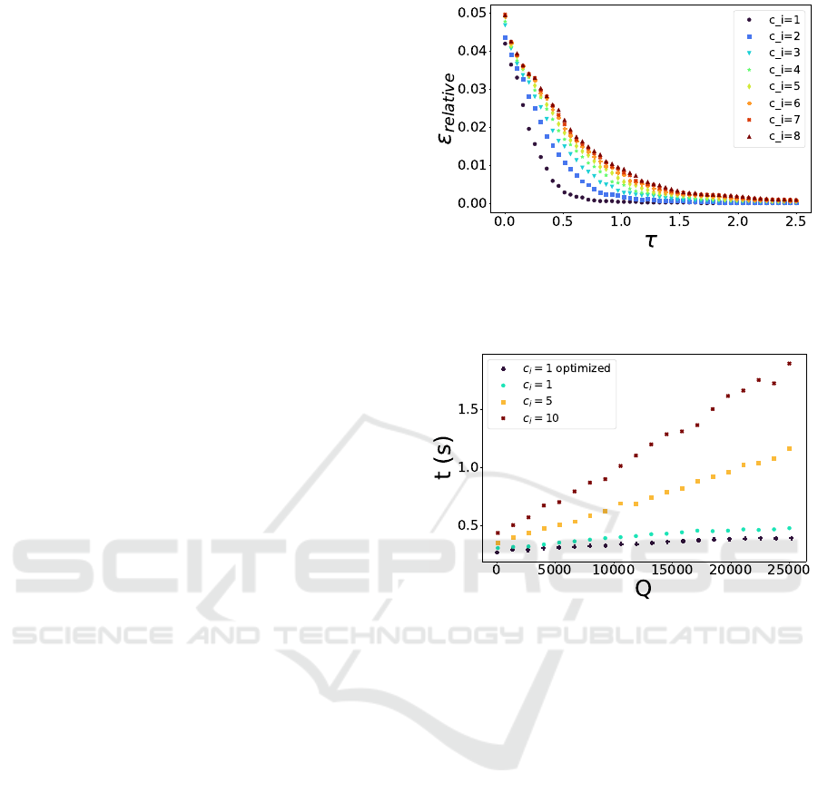
Figure 6: Knapsack problem: Relative error ε

relative

= 1 −

V (⃗x

)/V (⃗x

) depending on τ and c

. Each problem has

1000 classes and a capacity of 0.8

∑

n−1

i=0

Figure 7: Knapsack problem: Dependency between the ca-

pacity of the knapsack Q and the execution time for dif-

ferent problem instances. Use of intermediate calculations,

number of classes n = 5000, τ = 1.

4 RESULTS AND

COMPARATIVES

After explaining the theoretical framework of the al-

gorithms, we present a series of experiments to com-

pare our approaches with other classical algorithms.

We evaluate both, the quality of the solutions versus τ

and the execution time versus the size of the problem.

4.1 Knapsack Results

The original idea was to compare our algorithm with

the Google Or-tools solver. However, due to its lim-

itation of requiring v

to be integer and its signiﬁ-

cantly lower maximum weight capacity Q, we have

excluded this option. Therefore, the algorithm used

for the comparisons is a greedy approach, which is

capable of ﬁnding a good approximate solution in al-

most no time for every problem instance. Basically,

IQSOFT 2025 - 1st International Conference on Quantum Software

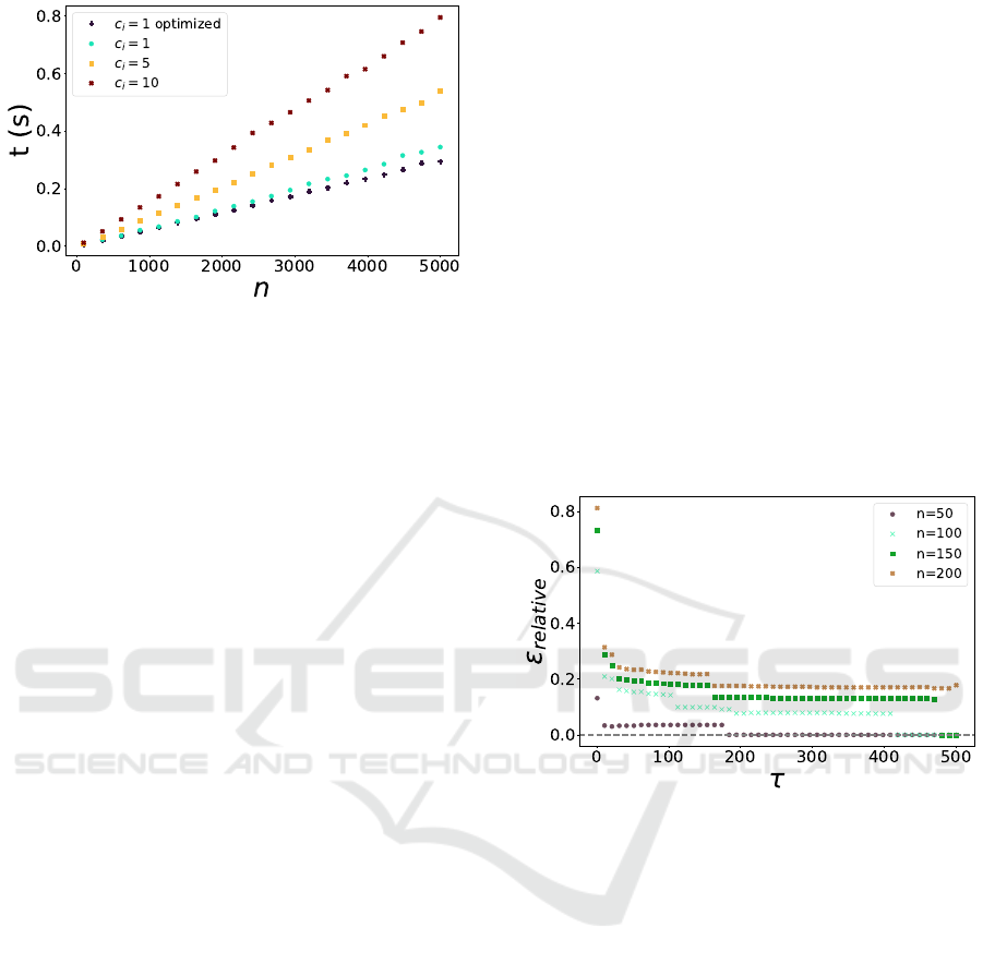
Figure 8: Knapsack problem: Dependency between the

number of classes n and the execution time for different

problem instances. Use of intermediate calculations, maxi-

mum weight capacity Q = 7000, τ = 1.

it consists of arranging the items in the knapsack in

ascending order according to the value/weight ratio,

and then inserting objects until the knapsack is ﬁlled

to the maximum. Fig. 6 displays how the algorithm

performs as a function of τ and the number of ele-

ments in all classes (in this case, all classes have the

same number of elements). Our indicator is the rel-

ative error ε

relative

= 1 −V (⃗x

)/V (⃗x

), being V(⃗x

)

the value of the tensor network solution and V (⃗x

)

the value of the greedy solution. As expected, as τ

increases, the relative error ε

relative

decreases, causing

the solution to approximate the greedy approach.

It should be noted that when τ reaches a certain

value, the product of the exponential may result in an

overﬂow, causing the algorithm to produce subopti-

mal solutions. This implies that, although this algo-

rithm is theoretically an exact method, in practice it is

not possible to solve arbitrarily large problems. When

exponential saturation is reached, the algorithm be-

gins to perform worse and, for this reason, it is crucial

to select a value τ that is large enough to distinguish

the optimal solution while remaining small enough to

prevent saturation.

Additionally, as mentioned in the theoretical sec-

tion, it is possible to verify in Figs. 7 and 8 that

by taking advantage of intermediate calculations, the

computational complexity in time of the algorithm de-

pends linearly with the maximum weight capacity Q

and the number of classes n. To avoid overﬂow, it

is possible to achieve better results using the Deci-

mal library. In fact, for problems with up to 1000

classes, our algorithm is able to ﬁnd better solutions

than greedy in several problem instances.

4.2 Shortest Path Problem

In order to compare how our algorithm performs

against Dijkstra’s (Dijkstra, 1959), we propose an

experiment where both algorithms have to go from

the same origin node to the same destiny node within

the same graph. This graph corresponds to Valladolid

city (Spain). Given that our algorithm needs to have

a ﬁxed number of steps in order to work, we compare

how the results evolve according to τ and the number

of steps. As can be seen in Fig. 9, both the number

of steps and the value of τ inﬂuence the result. The

higher the number of total steps, the greater τ needs to

be in order to reach the optimal solution. Our indica-

tor is the relative error ε

relative

= C(⃗x

)/C(⃗x

exact

)− 1,

being C(⃗x

) the value given by the tensor network

and C(⃗x

exact

) the number given by Dijkstra’s algo-

rithm. The relative error ε

relative

decreases as τ in-

creases, bringing the solution closer to the optimal.

Figure 9: Shortest path problem: Relative error ε

relative

C(⃗x

)/C(⃗x

exact

) − 1 depending on τ and n. Each problem

has V = 12408.

5 CONCLUSIONS

This work introduces a quantum-inspired tensor net-

work approach to solving the knapsack and the short-

est path problems. The methodology is based on some

quantum computing properties, such as superposition,

entanglement, or quantum measurements. Theoreti-

cally, the proposed algorithms allow to determine the

solutions of the problems exactly. However, due to

the overﬂow caused by the implementation, the efﬁ-

ciency of the algorithm is limited by the parameter τ

value. Even taking this into account, we have shown

that our algorithms are able to ﬁnd optimal solutions

for several problem instances (Figs. 7 and 8).

Future research will focus on analyzing the impact

of the parameter τ more systematically and develop-

ing alternative implementations that avoid numerical

Knapsack and Shortest Path Problems Generalizations from a Quantum-Inspired Tensor Network Perspective

overﬂows before reaching the optimal solution. Addi-

tionally, we aim to extend this approach to other com-

binatorial optimization problems, broadening the ap-

plicability of quantum-inspired tensor network meth-

ods in this domain, and study its possible implementa-

tion in quantum hardware to improve its performance.

ACKNOWLEDGMENT

The research has been funded by the Ministry of

Science and Innovation and CDTI under ECOSIS-

TEMAS DE INNOVACI

ON project ECO-20241017

(EIFEDE) and ICECyL (Junta de Castilla y Le

on) un-

der project CCTT5/23/BU/0002 (QUANTUMCRIP).

This proyect has been funded by the Spanish Min-

istry of Science, Innovation and Universities under

the project PID2023-149511OB-I00.

REFERENCES

Ali, A. M. (2025). Explicit solution equation for every com-

binatorial problem via tensor networks: Melocoton.

Ali, A. M., de Leceta, A. M. F., and Rubio, J. L. (2024a).

Anomaly detection from a tensor train perspective.

Ali, A. M., Delgado, I. P., and de Leceta, A. M. F. (2024b).

Traveling salesman problem from a tensor networks

perspective.

Ali, A. M., Delgado, I. P., Markaida, B. G., and de Leceta,

A. M. F. (2024c). Task scheduling optimization from

a tensor network perspective.

Ali, A. M., Delgado, I. P., Roura, M. R., and de Leceta, A.

M. F. (2024d). Polynomial-time solver of tridiagonal

qubo and qudo problems with tensor networks.

Bateni, M., Hajiaghayi, M., Seddighin, S., and Stein, C.

(2018). Fast algorithms for knapsack via convolution

and prediction. In Proceedings of the 50th Annual

ACM SIGACT Symposium on Theory of Computing,

STOC 2018, page 1269–1282, New York, NY, USA.

Association for Computing Machinery.

Benson, B. M., Ingman, V. M., Agarwal, A., and Keinan, S.

(2023). A cqm-based approach to solving a combina-

torial problem with applications in drug design.

Biamonte, J. (2020). Lectures on quantum tensor networks.

Biamonte, J. and Bergholm, V. (2017). Tensor networks in

a nutshell.

Dauz

ere-P

es, S., Ding, J., Shen, L., and Tamssaouet, K.

(2024). The ﬂexible job shop scheduling problem: A

review. European Journal of Operational Research,

314(2):409–432.

Dijkstra, E. W. (1959). A note on two problems in connex-

ion with graphs. Numerische Mathematik, 1(1):269–

271.

Egor, B., Egor, G., and Daria, L. (2022). Two heuristics for

one of bin-packing problems. IFAC-PapersOnLine,

55(10):2575–2580. 10th IFAC Conference on Man-

ufacturing Modelling, Management and Control MIM

2022.

Farhi, E., Goldstone, J., and Gutmann, S. (2014). A quan-

tum approximate optimization algorithm.

Fredman, M. L. and Tarjan, R. E. (1987). Fibonacci heaps

and their uses in improved network optimization algo-

rithms. J. ACM, 34(3):596–615.

Glover, F., Kochenberger, G., and Du, Y. (2019). A tutorial

on formulating and using qubo models.

Golub, G. and Kahan, W. (1965). Calculating the singular

values and pseudo-inverse of a matrix. Journal of the

Society for Industrial and Applied Mathematics Series

B Numerical Analysis, 2(2):205–224.

Gutin, G. and Yeo, A. (2007). The greedy algorithm for

the symmetric tsp. Algorithmic Operations Research,

2(1).

Hao, T., Huang, X., Jia, C., and Peng, C. (2022). A

quantum-inspired tensor network algorithm for con-

strained combinatorial optimization problems. Fron-

tiers in Physics, 10.

Hart, P. E., Nilsson, N. J., and Raphael, B. (1968). A for-

mal basis for the heuristic determination of minimum

cost paths. IEEE Transactions on Systems Science and

Cybernetics, 4(2):100–107.

Katangur, A., Pan, Y., and Fraser, M. (2002). Message rout-

ing and scheduling in optical multistage networks us-

ing simulated annealing. In Proceedings 16th Inter-

national Parallel and Distributed Processing Sympo-

sium, pages 8 pp–.

Korte, B. and Vygen, J. (2000). Bin-Packing, pages 407–

422. Springer Berlin Heidelberg, Berlin, Heidelberg.

Korte, B. and Vygen, J. (2008). The Traveling Salesman

Problem, pages 527–562. Springer Berlin Heidelberg,

Berlin, Heidelberg.

Laporte, G. (1992). The traveling salesman problem: An

overview of exact and approximate algorithms. Eu-

ropean Journal of Operational Research, 59(2):231–

247.

Lenstra, J. K. (1992). Job shop scheduling. In Akg

ul, M.,

Hamacher, H. W., and T

ufekc¸i, S., editors, Combina-

torial Optimization, pages 199–207, Berlin, Heidel-

berg. Springer Berlin Heidelberg.

Mathews, G. B. (1896). On the partition of numbers.

Proceedings of the London Mathematical Society, s1-

28(1):486–490.

Peruzzo, A., McClean, J., Shadbolt, P., Yung, M.-H., Zhou,

X.-Q., Love, P. J., Aspuru-Guzik, A., and O’Brien,

J. L. (2014). A variational eigenvalue solver on a pho-

tonic quantum processor. Nature Communications,

5(1):4213.

Pilcher, T. (2023). A self-adaptive genetic algorithm for the

ﬂying sidekick travelling salesman problem.

Qing, Y., Li, K., Zhou, P.-F., and Ran, S.-J. (2024). Com-

pressing neural network by tensor network with expo-

nentially fewer variational parameters.

Wang, B. and Dong, H. (2024). Bin packing optimization

via deep reinforcement learning.

Wang, J., Roberts, C., Vidal, G., and Leichenauer, S.

(2020). Anomaly detection with tensor networks.

CoRR, abs/2006.02516.

IQSOFT 2025 - 1st International Conference on Quantum Software