Lens Aberrations Detection and Digital Camera Identiﬁcation with

Convolutional Autoencoders

Jarosław Bernacki

1 a

and Rafał Scherer

2 b

Department of Artiﬁcial Intelligence, Cze¸stochowa University of Technology,

al. Armii Krajowej 36, 42-200 Cze¸stochowa, Poland

Faculty of Computer Science, AGH University of Krakow, Poland

Keywords:

Privacy, Security, Convolutional Neural Networks, Convolutional Autoencoders, Digital Forensics, Digital

Camera Identiﬁcation, Hardwaremetry.

Abstract:

Digital camera forensics relies on the ability to identify digital cameras based on their unique characteristics.

While many methods exist for camera ﬁngerprinting, they often struggle with efﬁciency and scalability due to

the large image sizes produced by modern devices. In this paper, we propose a novel approach that utilizes

convolutional and variational autoencoders to detect optical aberrations, such as vignetting and distortion.

Our model, trained in an aberration-independent manner, enables automatic detection of these distortions

without needing reference patterns. Furthermore, we demonstrate that the same methodology can be applied

to digital camera identiﬁcation based on image analysis. Extensive experiments conducted on multiple cameras

and images conﬁrm the effectiveness of our approach in both aberration detection and device ﬁngerprinting,

highlighting its potential applications in forensic investigations.

1 INTRODUCTION

Digital forensics is a ﬁeld that has garnered signif-

icant attention in recent years. One of the most

prominent topics in digital forensics is the identiﬁ-

cation of imaging sensors in digital cameras. Dig-

ital cameras have become widely accessible and af-

fordable, contributing to their popularity. Even more

prevalent are smartphones and mobile devices, com-

monly equipped with built-in digital cameras. This

widespread availability encourages people to take

photos and share them on social media networks.

However, the capability to determine whether an im-

age was taken by a speciﬁc camera can pose a seri-

ous threat to user privacy. Consequently, a substan-

tial body of research in recent years has focused on

studying imaging device artifacts that can be used for

digital camera identiﬁcation.

Digital camera identiﬁcation can be approached in

two primary ways: individual source camera identi-

ﬁcation (ISCI) and source model camera identiﬁca-

tion (SCMI). ISCI can distinguish a speciﬁc camera

among cameras of the same model and different mod-

els. In contrast, SCMI can only differentiate between

https://orcid.org/0000-0002-4488-3488

https://orcid.org/0000-0001-9592-262X

different camera models but not between individual

cameras of the same model. For example, given cam-

eras such as Canon EOS R (0), Canon EOS R (1), ...,

Canon EOS R (n), Nikon D780 (0), Nikon D780 (1),

Sony A1 (0), and Sony A1 (1), ISCI would differenti-

ate each camera, while SCMI would only identify the

general models (Canon EOS R, Nikon D780, Sony

A1). This limitation of SCMI motivates the develop-

ment of methods and algorithms focused on the ISCI

aspect.

The most common methods for digital camera

identiﬁcation are based on Photo-Response Non-

Uniformity (PRNU). These methods compare the

noise patterns of a given image with the known noise

pattern of a camera. PRNU arises from imperfections

in the image sensor, creating a unique pattern for each

camera. This pattern can be estimated from multiple

images captured by a camera and used as a reference

for identiﬁcation. If the PRNU patterns match, the

image was likely captured by that camera. PRNU-

based methods are widely used due to their robustness

against post-capture processing and compression.

A state-of-the-art algorithm for ISCI was pro-

posed by Luk’as et al. (Luk

as et al., 2006), utilizing

PRNU for camera identiﬁcation. The PRNU K may

be calculated in the following manner: K = I − F(I),

Bernacki, J. and Scherer, R.

Lens Aberrations Detection and Digital Camera Identiﬁcation with Convolutional Autoencoders.

DOI: 10.5220/0013485900003979

In Proceedings of the 22nd International Conference on Security and Cryptography (SECRYPT 2025), pages 84-95

ISBN: 978-989-758-760-3; ISSN: 2184-7711

where I is the input image and F is a denoising ﬁlter.

This PRNU acts as a unique ﬁngerprint for the cam-

era. Many studies have conﬁrmed the high efﬁcacy

of this method. However, a signiﬁcant drawback is

that the camera’s ﬁngerprint is represented as a ma-

trix with the original image dimensions, posing stor-

age challenges for large numbers of PRNUs in foren-

sic centers. This issue drives the need for methods to

minimize this storage problem.

Another approach involves feature-based meth-

ods, which extract features such as metadata, color

balance, geometric distortion, lens artifacts, etc.,

and match them with known camera features. The

most recent family of methods utilizes deep learning,

typically employing convolutional neural networks

(CNNs) to extract features from images and compare

them with features from known cameras (Bondi et al.,

2017; Ding et al., 2019; Kirchner and Johnson, 2020;

Li et al., 2018; Luk

as et al., 2006; Mandelli et al.,

2020; Yao et al., 2018). Additionally, various hybrid

methods combine multiple algorithms to enhance the

accuracy of camera identiﬁcation.

Lens aberration identiﬁcation is a critical aspect

of digital forensics. Despite technological advance-

ments, both digital single-lens reﬂex (DSLR) and

mirrorless cameras continue to suffer from various

optical issues. Common deviations include chro-

matic aberrations, dispersion, vignetting, distortion,

and coma. Vignetting, which can result from opti-

cal defects or sensor imperfections (Lopez-Fuentes

et al., 2015; Ray, 2002), is a reduction of the im-

age brightness near the edges, leading to darker cor-

ners. This ﬂaw is especially prevalent in compact and

DSLR cameras. Types of vignetting are thoroughly

detailed in (Lopez-Fuentes et al., 2015), and the prob-

lem has garnered signiﬁcant research attention, with

numerous algorithms (De Silva et al., 2016; Kordecki

et al., 2017) and patents (Lee et al., 2017) proposed

for its correction. Another related issue is lens dis-

tortion, which occurs as a deviation from rectilinear

projection (Park and Hong, 2001; Claus and Fitzgib-

bon, 2005). This distortion causes straight lines to ap-

pear curved in images and is characterized by changes

in magniﬁcation relative to the image’s distance from

the optical axis (Goljan and Fridrich, 2014).

1.1 Contribution

The contribution of this paper is twofold. Firstly, we

propose a method that utilizes a convolutional (CAE)

and variational (VAE) autoencoder to identify images

that show different types of lens aberrations, includ-

ing lens vignetting and distortion. We experimentally

show that our methods are capable of detecting lens

vignetting based on several models of lenses, as well

as detecting lens distortion with a reliable probabil-

ity. Secondly, we show that the proposed autoen-

coders may be used to identify digital cameras in the

ISCI aspect based on images. We demonstrate that

this approach requires less time for training, which

may speed up the image processing workﬂow. Our

experiments, conducted on a large set of modern dig-

ital cameras, conﬁrm that the accuracy of our method

is comparable to state-of-the-art methods. Addition-

ally, we perform a statistical analysis of the obtained

results, which further conﬁrms their reliability.

1.2 Organization of the Paper

The paper is organized as follows. The next section

discusses previous and related works. In Section 3

the problem formulation and the proposed method are

described. Section 4 presents the results of classiﬁca-

tion compared with the state-of-the-art methods. In

Section 5 there are described the results of statistical

analysis. The ﬁnal section concludes this work.

2 PREVIOUS AND RELATED

WORK

In (Baar et al., 2012), the authors proposed utilizing

the k-means algorithm to manage photo response non-

uniformity (PRNU) patterns. These patterns are com-

pared using correlation and then grouped by the k-

means algorithm. As a result, patterns grouped within

the same cluster are considered to belong to the same

camera. Experiments conducted on a database of 500

images showed that images within a cluster had a

true positive rate (TPR) of 98% for belonging to a

particular camera. In (Julliand et al., 2016), the au-

thors demonstrate that different types of noise signiﬁ-

cantly affect raw images. They show that JPEG lossy

compression generates noise that impacts groups of

pixels. A speciﬁc example highlighted how an im-

age’s histogram changes before and after saving it as

a JPEG, indicating that JPEG compression introduces

distinct artifacts that can be used for identiﬁcation

purposes. In (Taspinar et al., 2016), the feasibility

of sensor recognition for image blocks smaller than

50 × 50 pixels is explored. The study uses the peak-

to-correlation energy (PCE) ratio for veriﬁcation, and

results indicate that analyzing such small blocks with

low PCE values is inefﬁcient. The objective of (Jiang

et al., 2016) is to determine if images across several

social network accounts were taken by the same user.

The authors employ the formula from (Luk

as et al.,

2006) to ﬁnd the camera ﬁngerprint and cluster im-

Lens Aberrations Detection and Digital Camera Identiﬁcation with Convolutional Autoencoders

ages based on correlation. Experiments with 1576 im-

ages evaluated performance using precision and recall

measures, achieving a clustering precision of 85% and

a recall of 42%.

The analysis of how image features affect PRNU

is discussed in (Tiwari and Gupta, 2018). Intensity-

based features and high-frequency details, such as

edges and textures, impact the ﬁnal quality of the

camera’s ﬁngerprint. To enhance this quality, a

weighting function (WF) is proposed. Initially, re-

gions of the image that provide reliable and unre-

liable PRNU are estimated. Then, the WF assigns

higher weights to regions yielding reliable PRNU and

lower weights to those producing less reliable PRNU.

In (Marra et al., 2018), the vulnerability of deep learn-

ing approaches to adversarial attacks in digital cam-

era identiﬁcation is examined. The goal is to demon-

strate how to deceive a CNN-based classiﬁer to pro-

duce incorrect camera identiﬁcation. The study de-

scribes several scenarios where the image undergoes

lossless or lossy compression. Attacks on the clas-

siﬁer are performed using methods such as the Fast

Gradient Sign Method (FGSM)(Goodfellow et al.,

2015), DeepFool(Moosavi-Dezfooli et al., 2016), and

the Jacobian-based Saliency Map Attack (JSMA) (Pa-

pernot et al., 2016). FGSM involves adding additive

noise to the image, which can sometimes visibly af-

fect image quality. To mitigate this, DeepFool uses lo-

cal linearization of the classiﬁer under attack. JSMA,

on the other hand, is a greedy iterative procedure that

computes a saliency map at each iteration, identifying

the pixels that most inﬂuence correct classiﬁcation.

Experiments demonstrated that these attack methods

can effectively deceive CNN-based classiﬁers.

3 PROPOSED AUTOENCODERS

3.1 Preliminaries and Problem

Formulation

Camera’s Fingerprint. Let M be the number of

images from camera A

(i)

. In order to learn the speci-

ﬁcity of the camera (but not the content of the input

image), we denoise the cameras’ images. We use

the well-known formula presented as eq. 1, utilized

in (Luk

as et al., 2006; Tuama et al., 2016) to calculate

the residuum K

for the j-th image of camera A

(i)

= I

− F(I

) (1)

where I

is the j-th image of camera A

(i)

, and F stands

for a denoising ﬁlter. To obtain the ﬁngerprint K

(i)

the camera A

(i)

we calculate:

(i)

∑

k=1

(i)

(2)

According to (Luk

as et al., 2006), the procedure de-

scribed as eq. 2 is representative, if M > 45.

Camera Identiﬁcation. Let us deﬁne the camera

identiﬁcation task as the statistical approach.

Deﬁnition 1. (Camera identiﬁcation task) Let N be

the number of cameras. For the image I deﬁne, from

which camera A

(i)

(where i ∈ {1, 2, . . ., N}) this image

comes from. We deﬁne the following hypotheses:

• The null hypothesis (H

): The image I comes

from the camera A

(i)

;

• The alternative hypothesis (H

): The image I does

not come from the camera A

(i)

To verify the hypotheses we have to deﬁne the sta-

tistical test T (I), which measures the compatibility of

the ﬁngerprint K

(i)

from the camera A

(i)

with a new

residuum K

(eq. 3):

T (I) = D(K

(i)

, K

) (3)

where D may be a distance function or correlation co-

efﬁcient. We reject the null hypothesis H

, whether:

T (I) > τ (4)

where τ is a rejection threshold (the critical value) on

the signiﬁcance level α.

The image I is considered as made with the cam-

era A

(i)

, if the test statistic meets the criterion:

T (I) ≤ τ (5)

If for all cameras T (I) > τ, then the image I was not

made by any of the considered cameras.

Aberrations. In this paper, we consider the follow-

ing lens aberrations: vignetting and distortion. Lens

vignetting is a defect that manifests itself as a de-

crease in the brightness of an image, usually in all its

corners relative to the center (Lanh et al., 2007; Ko-

rdecki et al., 2015). Formally, lens vignetting can be

modeled as presented in Def. 2.

Deﬁnition 2. (Lens vignetting) Let I

, y

) denote

the brightness in the middle of the image I. The vi-

gnetting may be deﬁned as the following:

I(r

(v)

) = I



1 − k ·



(v)

max

(v)





(6)

where:

• I(r

(v)

) – brightness in a selected pixel with r

(v)

distance from the middle of the image I;

SECRYPT 2025 - 22nd International Conference on Security and Cryptography

• I

, y

) – brightness in the middle of the image

• k – vignetting coefﬁcient;

• r

max

(v)

– maximum distance from the middle of the

image I.

The r

(v)

may be calculated using the Euclidean

distance r

(v)

(x − x

)

+ (y −y

)

for any pixel

(x, y).

Lens distortion is an optical defect that is visible in

photos as a distortion of shapes due to deviation from

a rectilinear projection (e.g. the edge of a building

in a distorted photo appears to be deviated from the

vertical, etc.). The most common types of distortion

are barrel distortion and pincushion distortion. In bar-

rel distortion, the center of the frame is emphasized,

while in pincushion distortion, the center of the frame

looks “sunken” (Goljan and Fridrich, 2014). Simpli-

fying a bit, distortion occurs when lines created by

pixels, which in the real world should be vertical or

horizontal, are not parallel to its edges or are curved in

the photo. Formally, lens distortion can be described

as in Def. 3.

Deﬁnition 3. (Lens distortion) For an image without

distortion, the pixel coordinates (x, y) are mapped to

the coordinates (x

′

, y

′

) in the distorted image accord-

ing to the equation:

′

(d)

= r

(d)

· (1 +k

(d)

+ k

(d)

) (7)

where:

• r

(d)

is the distance of the pixel from the center of

the image;

• k

, k

– distortion coefﬁcients;

• r

′

(d)

– the distance of the distorted pixel from the

center.

Let us deﬁne the task of aberration detection,

which is considered as lens vignetting and lens distor-

tion detection, using the convolutional autoencoder.

Deﬁnition 4. (Aberration detection) Let D =

, Y

}

j=1

denote the training set. The I

is an in-

put image, and Y

denotes the mask corresponding to

the image I

, where each value y

∈ {0, 1} represents

every pixel of I

if it shows the aberration (1) or not

(0). The I

has dimensions H ×W × C, where H is

the image height, W stands for the image width and

C is the number of color channels (typically for RGB

images C = 3).

Let f

be the convolutional autoencoder with pa-

rameters θ. The autoencoder f

transforms the im-

age I

into the matrix of predictions

, where

). The dimensions of

are H × W , where

ˆy

∈ [0, 1] is the probability that the k-th pixel shows

the aberration.

Deﬁnition 5. (Loss function) For the image I

the bi-

nary cross-entropy function is deﬁned as:

Λ(I

, Y

) = −

H×W

∑

k=1

log( ˆy

(1 − y

)log(1 − ˆy

)]

(8)

where:

• y

is the label for the pixel k;

• ˆy

is the probability for the pixel k;

• H and W are dimensions of the image I

Deﬁnition 6. (Minimizing the loss function) During

the training the parameters θ are optimized, minimiz-

ing the loss function:

min

∑

j=1

Λ(I

, Y

) (9)

As the optimization algorithm, Adam (Kingma

and Ba, 2015) is used.

Deﬁnition 7. (Aberration prediction) The autoen-

coder f

generates for the new image I

the matrix

of predictions

= f

). To receive the ﬁnal de-

cision on aberration, the thresholding is used in the

following manner:

ˆy

x,k

(

1 if ˆy

x,k

≥ γ

0 if ˆy

x,k

< γ

where γ is a threshold, for instance γ = 0.5 decides if

the pixel k is marked as aberrated (1) or not (0).

3.2 The Proposed Autoencoders

Convolutional Autoencoder. The convolutional

autoencoder (CAE) is a classic autoencoder approach

that consists of two main parts: the encoder (encod-

ing part), and the decoder (the decoding part). The

encoder reduces the input resolution gradually as the

number of channels increases. The decoder, con-

versely, restores the original resolution. We propose

the following structure of the CAE:

The encoding part:

(1) A ﬁrst convolutional layer of 32 ﬁlters of size 3 ×

3 (stride 2), with ReLU as an activation function,

followed by a Max-Pooling layer + padding 1;

(2) A second convolutional layer of 64 ﬁlters of

size 3 × 3 (stride 2), with ReLU as an activa-

tion function, followed by a Max-Pooling layer +

padding 1;

(3) A third convolutional layer of 128 ﬁlters of size

3 × 3 (stride 2), with ReLU as an activation

function, followed by a Max-Pooling layer +

padding 1;

Lens Aberrations Detection and Digital Camera Identiﬁcation with Convolutional Autoencoders

(4) A fourth convolutional layer of 256 ﬁlters of

size 3 × 3 (stride 2), with ReLU as an activa-

tion function, followed by a Max-Pooling layer +

padding 1.

The decoding part:

(1) A ﬁrst transposed convolutional layer of 128 ﬁl-

ters of size 3 × 3 (stride 2), with ReLU as an acti-

vation function, followed by a Max-Pooling layer

+ padding 1;

(2) A second transposed convolutional layer of 64 ﬁl-

ters of size 3 × 3 (stride 2), with ReLU as an acti-

vation function, followed by a Max-Pooling layer

+ padding 1;

(3) A third transposed convolutional layer of 32 ﬁl-

ters of size 3 × 3 (stride 2), with ReLU as an acti-

vation function, followed by a Max-Pooling layer

+ padding 1;

(4) A fourth transposed convolutional layer with a ﬁl-

ter of size 3× 3 (stride 2), with sigmoid as an acti-

vation function, followed by a Max-Pooling layer

+ padding 1.

The encoder consists of four convolutional layers,

which gradually reduce the image resolution and in-

crease the number of channels. Each convolutional

layer acts as a ﬁlter, capturing increasingly abstract

features – from edges and textures to more complex

structures. As we go through the layers, information

about details is lost, but important features are pre-

served, representing the image in a compressed way.

After the last layer, we get a low-dimensional repre-

sentation (so-called latent vector).

The decoder reverses the encoder’s operation – it

uses transposed convolutional layers (deconvolution)

to restore the original image size. Each step gradually

increases the resolution, reconstructing missing de-

tails. The ﬁnal layer returns an image in the range of

values [0,1], usually using a sigmoid activation func-

tion. The model learns to minimize the difference be-

tween the input and the output, so it can effectively

eliminate noise or detect anomalies when the recon-

struction does not match the input (e.g. distortion or

vignetting).

Variational Autoencoder. The structure of the vari-

ational autoencoder (VAE) is generally similar to the

structure of CAE, but additionally, the VAE uses lin-

ear layers (fully connected) to encode an image into

the latent vector. Let us discuss the proposed VAE

with the following structure:

The encoding part:

(1) A ﬁrst convolutional layer of 32 ﬁlters of size 3 ×

3 (stride 2), with ReLU as an activation function,

followed by a Max-Pooling layer + padding 1;

(2) A second convolutional layer of 64 ﬁlters of

size 3 × 3 (stride 2), with ReLU as an activa-

tion function, followed by a Max-Pooling layer +

padding 1;

(3) A third convolutional layer of 128 ﬁlters of size

3 × 3 (stride 2), with ReLU as an activation

function, followed by a Max-Pooling layer +

padding 1;

(4) A fourth convolutional layer of 256 ﬁlters of

size 3 × 3 (stride 2), with ReLU as an activa-

tion function, followed by a Max-Pooling layer +

padding 1;

(5) Fully connected layers which generate the µ

(mean) and logvar (log variance) parameters to

model the latent vector.

The decoding part:

(1) A ﬁrst transposed convolutional layer of 128 ﬁl-

ters of size 3 × 3 (stride 2), with ReLU as an acti-

vation function, followed by a Max-Pooling layer

+ padding 1;

(2) A second transposed convolutional layer of 64 ﬁl-

ters of size 3 × 3 (stride 2), with ReLU as an acti-

vation function, followed by a Max-Pooling layer

+ padding 1;

(3) A third transposed convolutional layer of 32 ﬁl-

ters of size 3 × 3 (stride 2), with ReLU as an acti-

vation function, followed by a Max-Pooling layer

+ padding 1;

(4) A fourth transposed convolutional layer with a ﬁl-

ter of size 3× 3 (stride 2), with sigmoid as an acti-

vation function, followed by a Max-Pooling layer

+ padding 1.

Similar to a classic autoencoder, the encoder con-

sists of convolutional layers that reduce the image res-

olution and extract key features. However, instead of

returning a latent vector, the model generates two vec-

tors – µ (mean) and logvar (log variance), which de-

ﬁne a normal distribution in the latent vector. Instead

of direct encoding, the model samples values from

this distribution (using reparameterization), which in-

troduces an element of randomness and allows the

generation of new images.

The decoder works similarly to CAE, but instead

of reconstructing the image from a latent vector, it

does so from a sample taken from a Gaussian distri-

bution. This allows the model to generate diverse im-

ages, even if the input image is the same. The decoder

gradually increases the resolution through transposed

convolutional layers and ends with a layer with sig-

moid activation, returning the image reconstruction.

SECRYPT 2025 - 22nd International Conference on Security and Cryptography

The Discriminator. In order to classify images, the

discriminator may be used. The idea of the discrimi-

nator is based on the Generative Adversarial Network

(GAN) (Goodfellow et al., 2014). The use of the

discriminator is essential to classify the images pro-

duced by autoencoder decoders. We propose to use

as the discriminator a convolutional neural network,

however, well-known machine learning algorithms,

such as Support Vector Machine (SVM) might also

be used.

The structure of the sample discriminator is described

below:

(1) A ﬁrst convolutional layer of 32 ﬁlters of size 3 ×

3 with ReLU as an activation function, stride 2,

followed by a max-pooling layer;

(2) A second convolutional layer of 64 ﬁlters of size

3 × 3 with ReLU as an activation function, stride

2, followed by a max-pooling layer;

(3) A third convolutional layer of 128 ﬁlters of size

3 × 3 with ReLU as an activation function, stride

2, followed by a max-pooling layer;

(4) Fully connected 512 + dropout 0.5 + ReLU;

(5) Fully connected 128 + dropout 0.5.

The activation function is softmax.

All meta-parameters both for the proposed autoen-

coders, as well the discriminator were determined ex-

perimentally.

4 EXPERIMENTAL EVALUATION

We conduct two experiments. The ﬁrst experiment

presents the results of lens aberrations detection, in-

cluding vignetting and distortion identiﬁcation with

the proposed autoencoders. The second experiment

shows the standard identiﬁcation procedure for both

of the proposed CAE and VAE, as well as considered

state-of-the-art methods.

4.1 Experimental Setup

Datasets. For both experiments, we use images

coming from the IMAGINE dataset (Bernacki. and

Scherer., 2023).

For experiment I, we use both images from

the IMAGINE dataset but also blank images that

may make learning the lens vignetting and lens

distortion. Firstly, the autoencoders are trained with

aberration-free images. To determine whether the

images have distorted pixels, we have used the Hugin

Photo Stitcher software (hug, enet). For each case

(no vignetting; not distorted) at least 30 images were

used (per lens). Sample images used for training are

shown as Fig. 1 and 2. The following cameras and

lenses were used for the Experiment I:

Nikon D3100:

1. Nikon Nikkor AF-S DX 18-105 mm f/3.5-5.6 VR

2. Nikon Nikkor AF-S DX 35 mm f/1.8G

Nikon D7200:

1. Nikon Nikkor AF-P DX 10-20 mm f/4.5-5.6G VR

2. Nikon Nikkor AF-S DX 18-55 mm f/3.5-5.6G VR

3. Nikon Nikkor AF-S DX Micro 40 mm f/2.8G

Nikon D750:

1. Nikon Nikkor AF-S 20 mm f/1.8G ED

2. Nikon Nikkor AF 50 mm f/1.8D

Panasonic GX80:

1. Panasonic G VARIO 14-42 mm f/3.5-5.6 MEGA

O.I.S

2. Olympus M.Zuiko Digital ED 30 mm f/3.5 Macro

For experiment II, we use a set of 17 modern cam-

eras that include Canon EOS 1D X Mark II (C1),

Canon EOS 5D Mark IV (C2), Canon EOS M5 (C3),

Canon EOS M50 (C4), Canon EOS R (C5), Canon

EOS R6 (C6), Canon EOS RP (C7), Fujiﬁlm X-T200

(F1), Nikon D5 (N1), Nikon D6 (N2), Nikon D500

(N3), Nikon D780 (N4), Nikon D850 (N5), Nikon

Z6 II (N6), Nikon Z7 II (N7), Sony A1 (S1), Sony

A9 (S2). At least 30 images per camera are used for

learning.

Evaluation Measures. As evaluation, we use stan-

dard accuracy (ACC), deﬁned as:

ACC =

TP + TN

TP + TN + FP + FN

where TP/TN denotes “true positive/true negative”;

FP/FN stands for “false positive/false negative”. TP

denotes the number of cases correctly classiﬁed to a

speciﬁc class; TN refers to instances that are correctly

rejected. FP denotes cases incorrectly classiﬁed to the

speciﬁc class; FN is cases incorrectly rejected.

Implementation. Experiments are held on a Gi-

gabyte Aero notebook equipped with an Intel Core

i7-13700H CPU with 32 gigabytes of RAM and a

Nvidia GeForce RTX 4070 GPU with 8 gigabytes of

video memory. Scripts for CNNs are implemented

in Python under the PyTorch framework (with Nvidia

CUDA support).

Lens Aberrations Detection and Digital Camera Identiﬁcation with Convolutional Autoencoders

(a) (b) (c)

Figure 1: Sample images for lens vignetting identiﬁcation: (a) – blank vignetted image; (b) and (c) – blank and natural

(respectively) non-vignetted images (Nikon D750 + Nikon Nikkor AF-S 20 mm f/1.8G ED).

(a) (b)

Figure 2: Sample images for lens distortion identiﬁcation:

(a) – distorted image; (b) – non-distorted image (Nikon

D3100 + Nikon Nikkor AF-S DX 18-105 mm f/3.5-5.6 VR

ED).

4.2 State-of-the-Art Methods – Recall

Let us recall some methods for a digital camera iden-

tiﬁcation.

Mandelli et al.’s CNN. Let us brieﬂy recall the

structure of Mandelli et al.’s (Mandelli et al., 2020)

convolutional neural network (CNN):

(1) A ﬁrst convolutional layer of kernel 3 × 3 produc-

ing feature maps of size 16×16 pixels with Leaky

ReLU as an activation method and max-pooling;

(2) A second convolutional layer of kernel 5 × 5 pro-

ducing feature maps of size 64 × 64 pixels with

Leaky ReLU as an activation method and max-

pooling;

(3) A third convolutional layer of kernel 5×5 produc-

ing feature maps of size 64×64 pixels with Leaky

ReLU as an activation method and max-pooling;

(4) A pairwise correlation pooling layer;

(5) Fully connected layers (FC).

For more details related to the structure of the net-

work, we refer to the authors’ paper.

Kirchner & Johnson’s CNN. Kirchner and John-

son (Kirchner and Johnson, 2020) proposed a follow-

ing network:

1. 17 layers implementing 64 convolutional ﬁlters

with 3 × 3 kernels;

2. ReLU as an activation method after each layer;

3. Fully connected layers (FC).

All aforementioned convolutional neural networks

are trained by noise residuals calculated with the de-

noising formula (Eq. 10).

Luk

as et al.’s Algorithm. The non-convolutional

Luk

as et al.’s algorithm (Luk

as et al., 2006) is based

on the calculation of the noise residual K as shown in

Equation 10.

K = I − F(I), (10)

where F is a denoising (usually wavelet-based) ﬁlter,

the K stands for a single noise residual of one image I.

To obtain a representative noise residual of the cam-

era, this procedure should be repeated for at least 45

images. The camera’s noise residual is ﬁnally calcu-

lated as an average of a particular number of single

noise residuals. It is recommended to process images

in their original resolution.

4.3 Experiment I – Detecting Lens

Aberrations

In this experiment, we tested our proposed autoen-

coders to see if they were capable of detecting images

with lens aberrations that were considered vignetting

and distortion. The CAE and VAE were trained both

the non-vignetted and undistorted images I

. After

training, the new test images representing aberrations

were passed to the autoencoders in order to recon-

struct a new image I

. We have analyzed the mean

squared error (MSE, eq. 11) between the reconstruc-

tion of aberrated I

and I

images.

MSE =

∑

i=1

∑

j=1



(i, j)− I

(i, j)



(11)

According to our experiments, if MSE > 10, we

interpreted that CAE/VAE detected the aberration.

Otherwise, the aberration was not detected. The M

and N stand for images dimensions (in pixels).

SECRYPT 2025 - 22nd International Conference on Security and Cryptography

Lens Vignetting Detection. The results of the vi-

gnetting detection for the CAE and VAE autoencoders

are presented in Tab. 1 and 2.

Table 1: CAE: Results of classifying the images that repre-

sent vignetting for all used cameras and lenses [%].

vignetted non-vignetted

vignetted 83.0 17.0

non-vignetted 10.0 90.0

Table 2: VAE: Results of classifying the images that repre-

sent vignetting for all used cameras and lenses [%].

vignetted non-vignetted

vignetted 89.0 11.0

non-vignetted 6.0 94.0

The average accuracy of the proposed autoen-

coders for classifying both vignetting and non-

vignetting images is 89.0%. In the case of CAE,

vignetted images are correctly identiﬁed in 83.0%,

meaning that some images (17.0%) are not detected.

The VAE performs even better, achieving 89.0% in

recognizing vignetted images. Both models per-

form slightly better in recognizing non-vignetting im-

ages, correctly classifying 90.0% (CAE) and 94.0%

(VAE) of them. However, there are still false posi-

tives, meaning that some non-vignetting images are

incorrectly labeled as vignetting. Overall, both mod-

els show satisfactory performance but may require

further improvements to better distinguish between

difﬁcult-to-classify cases.

Lens Distortion Detection. The results of the dis-

tortion detection for both autoencoders are presented

in Tab. 3 and 4.

Table 3: CAE: Results of classifying the images that repre-

sent distortion for all used cameras and lenses [%].

distorted non-distorted

distorted 87.0 13.0

non-distorted 11.0 89.0

Table 4: VAE: Results of classifying the images that repre-

sent distortion for all used cameras and lenses [%].

distorted non-distorted

distorted 92.0 8.0

non-distorted 7.0 93.0

In the case of distortion recognition, the average

accuracy of the proposed autoencoders is also equal

to 90.25%. These results indicate that the proposed

models offer reliable results of lens distortion detec-

tion. The test images representing the distortion were

correctly identiﬁed in 87.0% and 92.0% of instances

for CAE and VAE, respectively. However, 13.0% and

8.0% were incorrectly identiﬁed as non-distorted. On

the other hand, 89.0% of non-distorted test images

were correctly detected (CAE); 93.0% is the result

of the VAE. Similarly, as in the case of vignetting,

some images were incorrectly classiﬁed as distorted

images.

4.4 Experiment II – Results of Digital

Camera Identiﬁcation

We have also tested, if the proposed autoencoders

may realize the task of camera identiﬁcation based on

images. However contrary to Experiment I, the us-

age of CAE and VAE were changed. We have used

only the encoder part of both autoencoders in order

to generate the latent vectors. Then, the discriminator

(introduced in subsec. 3.2) was trained with the latent

vectors and made the ﬁnal classiﬁcation. In this ex-

periment, all the tested methods were trained with the

noise residuals calculated in the manner as shown in

Eq. 10. Due to paper limitations, we skip presenting

confusion matrices of cameras’ classiﬁcation results.

The shortened results of classiﬁcation are presented

in Tab. 5.

Table 5: Results of classiﬁcation.

Method ACC [%]

CAE 91.0

VAE 89.0

Mandelli 92.0

Kirchner 92.0

Luk

as 92.0

The results clearly indicate that all methods en-

sure very high identiﬁcation accuracy. The proposed

CAE achieves 91.0% identiﬁcation accuracy, and the

VAE 89.0%. In the other cases, the overall iden-

tiﬁcation accuracy obtains at least 92.0%; the par-

ticular TPs are not lower than 90.0% for each cam-

era. The Luk

as et al.’s algorithm achieves almost the

same results compared to CNN-based methods. This

clearly conﬁrms that all methods ensure reliable in-

dividual source camera identiﬁcation. In the case of

the discussed CNNs, the results are very similar to

each other both in terms of identiﬁcation accuracy and

speed of learning.

All the methods require a similar number of train-

ing epochs to obtain the desired level of identiﬁcation

accuracy, which in this case was set to 2000. The

learning rate was equal to 0.01, the Adam optimizer

was used.

Lens Aberrations Detection and Digital Camera Identiﬁcation with Convolutional Autoencoders

Speed of Learning. We have compared the time

needed for training the proposed autoencoders and

CNN-based methods. Results may be seen in Fig. 3.

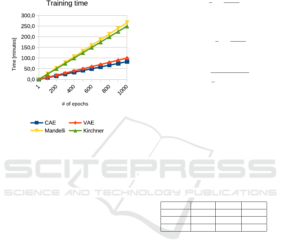
Figure 3: Comparison of time needed for learning 1000

epochs.

Results indicate that training the CAE and VAE

requires less time per epoch than using state-of-the-art

CNNs. One epoch using the proposed AEs is passed

over 0.1 of a minute while using CNN turns to about

0.3 of a minute. Therefore, the overall time for pass-

ing 1000 epochs requires about 100 minutes for the

proposed AEs and at least 250 minutes (more than 4

hours) for CNNs. Thus, it conﬁrms the advantages

over the literature methods.

5 STATISTICAL VERIFICATION

– EXPERIMENT II

In this section, we analyze the TP values between

the proposed autoencoders, Mandelli, Kirchner, and

Luk

as et al.’s algorithms. We determine whether there

exist signiﬁcant differences in this data. For this pur-

pose, we analyze the MAE, MAPE, and RMSE error

values, as well as the statistical veriﬁcation of the de-

ﬁned hypotheses. The statistical veriﬁcation concerns

the results presented in Experiment II.

5.1 Error Analysis

We compare the TPs obtained by the proposed

method and state-of-the-art methods by calculat-

ing estimators including mean absolute error (MAE,

eq. 12), mean absolute percentage error (MAPE,

eq. 13) and root mean square error (RMSE, eq. 14).

MAE =

∑

t=1



− x



(12)

where x

is the actual value, y

is a predicted value and

n is the number of observations.

MAPE = 100

∑

t=1



− y



(13)

where x

is the actual value, y

is a predicted value and

n is the number of observations.

RMSE =

∑

t=1



− y



(14)

where x

is the actual value, y

is a predicted value and

n is the number of observations.

The results conﬁrm that the classiﬁcation using

the proposed autoencoders achieves similar results as

state-of-the-art algorithms. The MAE values obtain

1.05-1.12; the RMSE receives from 1.23 to 1.47, and

the MAPE measure reaches from 1.15 to 1.20. Such

small values mean that TP results obtained by the pro-

posed autoencoders compared with other methods do

not differ more than 1.20%. Also, none of the mea-

sures exceed 1.47, which we ﬁnd satisfactory. The

results of the analysis are shown in Tab. 6.

Table 6: The values of MAE, MAPE, and RMSE measures

of the proposed CAE/VAE against state-of-the-art methods.

MAE MAPE RMSE

Mandelli 1.0588 1.1483 1.3284

Kirchner 1.0588 1.1510 1.2367

Luk

as 1.1176 1.2034 1.4753

5.2 Hypotheses Veriﬁcation

We have checked if there exists a statistical differ-

ence between the results of classiﬁcation by the CAE,

VAE, and methods by Mandelli, Kirchner, and Luk

as.

All tests were performed at the signiﬁcance level α =

0.05. The ﬁrst step is the normality test. The hypothe-

ses are deﬁned as follows:

• H

: Data represent the normal distribution;

• H

: Data does not represent the normal distribu-

tion.

We use the single-sample Shapiro-Wilk (SW) test.

Results are presented in Tab. 7.

SECRYPT 2025 - 22nd International Conference on Security and Cryptography

Table 7: Normality test results. The p-value less than the

signiﬁcance level leads to the rejection of the null hypothe-

sis.

Data p-value test statistic S

CAE 0.001 0.771

VAE 0.002 0.792

Mandelli 0.004 0.817

Kirchner 0.004 0.817

Luk

as 0.004 0.817

The critical values for a population consisting of

17 samples is S

= 0.892. To assume compliance with

a normal distribution test, the test statistic S should be

greater than S

. However, since S < S

for all consid-

ered data, we reject the null hypothesis about the nor-

mality of analyzed data. It is also conﬁrmed by the

p-values, which are much smaller than the considered

signiﬁcance level. Therefore, for further analysis,

we use the Kruskal–Wallis ANOVA non-parametric

test. The Kruskal-Wallis ANOVA test (also called

the Kruskal-Wallis one-way analysis of variance for

ranks) is an extension of the U Mann-Whitney test to

more than two populations. This test is used to verify

the hypothesis about the insigniﬁcance of differences

between the medians of the studied variable in sev-

eral (k > 2) populations (Kruskal and Wallis, 1952;

Kruskal, 1952). Its hypotheses are deﬁned as follows:

• H

: Medians θ

= θ

= . . . = θ

of the data are

equal;

• H

: Not all medians θ

(for n = 1, 2, . . .) of the

data are equal;

The test statistic is calculated as shown in Eq. 15.

H =

N(N + 1)

∑

i=1





∑

i=1

i j





− 3(N + 1) (15)

where:

• N =

∑

j=1

;

• n

– population cardinality (for j = 1, 2, . . . , k),

corresponding to the TP values of the CAE, VAE,

Mandelli, Kirchner, and Luk

as;

• R

i j

– ranks assigned to the variable value (i =

1, 2, . . . , n

, j = 1, 2, . . . , k).

The statistic has a χ

distribution with k − 1 de-

grees of freedom. First of all, let us calculate the

sum of ranks. For N =

∑

j=1

, we have k = 5;

= n

− n

= 17, therefore we obtain:

N = 5 · 17 = 85. The sum of ranks is presented in

Tab. 8.

Table 8: Sum of ranks for the Kruskal–Wallis ANOVA.

Data Sum of rangs

CAE 611.5

VAE 685.0

Mandelli 892.0

Kirchner 782.0

Luk

as 684.5

Next, let us calculate the test statistic for the TP

values obtained by the CAE, VAE, Mandelli, Kirch-

ner, and Luk

as:

H =

85(85 + 1)



611.5

685.0

892.0

782.0

684.5



− 3(85 + 1) = 1.58

Thus, the statistical test value of ANOVA analysis

for the CAE, VAE, Mandelli, Kirchner, and Luk

as is

equal to H = 1.58. The critical value of χ

distribu-

tion for 4 degrees of freedom is equal to F

= 9.49.

Because

F < F

there is no reason to reject the null hypothesis about

the equality of analyzed medians. Therefore, there

is no statistical difference between the proposed

CAE/VAE, Mandelli, Kirchner, and Luk

as. This may

be interpreted that all considered methods follow the

same high identiﬁcation accuracy.

Summary. The veriﬁcation of the obtained results

using both MAE, MAPE, and RMSE measures, and

hypotheses veriﬁcation conﬁrmed that the proposed

CAE and VAE make it possible to identify cameras

based on images with similar accuracy to state-of-the-

art methods. The MAE, MAPE, and RMSE mea-

sures represent small values, thus it may be inter-

preted that differences between each data are negligi-

ble. Also, the hypotheses veriﬁcation, using Kruskal-

Wallis ANOVA revealed that there is no statistical dif-

ference between the results of the classiﬁcation of the

proposed method and the literature’s methods, so one

may assume that the classiﬁcation is at the same level.

6 CONCLUSION

In this paper, we have proposed a method both for

lens aberrations detection, as well individual source

camera identiﬁcation based on images. The solu-

tion was based on convolutional and variational au-

toencoders. Extensive experimental evaluation con-

ducted on a large number of modern imaging devices

Lens Aberrations Detection and Digital Camera Identiﬁcation with Convolutional Autoencoders

conﬁrmed the high lens aberrations identiﬁcation ac-

curacy. Moreover, the proposed autoencoders may

be successfully used for digital camera identiﬁcation.

The experiments, enhanced with statistical analysis,

conﬁrmed the high identiﬁcation accuracy compared

with state-of-the-art methods. Additionally, experi-

ments revealed that using proposed autoencoders may

even shorten the processing time by up to half.

In future work, we consider an extended autoen-

coder model for increasing the accuracy of lens aber-

ration detection. We are also interested in identifying

different types of aberrations, including dispersion,

coma, and astigmatism.

REFERENCES

(http://hugin.sourceforge.net/). Hugin photo

stitcher.

Baar, T., van Houten, W., and Geradts, Z. J. M. H.

(2012). Camera identiﬁcation by grouping images

from database, based on shared noise patterns. CoRR,

abs/1207.2641.

Bernacki., J. and Scherer., R. (2023). Imagine dataset: Digi-

tal camera identiﬁcation image benchmarking dataset.

In Proceedings of the 20th International Conference

on Security and Cryptography - SECRYPT, pages

799–804. INSTICC, SciTePress.

Bondi, L., Barofﬁo, L., Guera, D., Bestagini, P., Delp,

E. J., and Tubaro, S. (2017). First steps toward cam-

era model identiﬁcation with convolutional neural net-

works. IEEE Signal Process. Lett., 24(3):259–263.

Claus, D. and Fitzgibbon, A. W. (2005). A rational function

lens distortion model for general cameras. In 2005

IEEE Computer Society Conference on Computer Vi-

sion and Pattern Recognition (CVPR’05), volume 1,

pages 213–219. IEEE.

De Silva, V., Chesnokov, V., and Larkin, D. (2016). A novel

adaptive shading correction algorithm for camera sys-

tems. Electronic Imaging, 28:1–5.

Ding, X., Chen, Y., Tang, Z., and Huang, Y. (2019). Cam-

era identiﬁcation based on domain knowledge-driven

deep multi-task learning. IEEE Access, 7:25878–

25890.

Goljan, M. and Fridrich, J. (2014). Estimation of lens

distortion correction from single images. In Media

Watermarking, Security, and Forensics 2014, volume

9028, pages 234–246. SPIE.

Goodfellow, I. J., Pouget-Abadie, J., Mirza, M., Xu, B.,

Warde-Farley, D., Ozair, S., Courville, A. C., and

Bengio, Y. (2014). Generative adversarial nets. In

Ghahramani, Z., Welling, M., Cortes, C., Lawrence,

N. D., and Weinberger, K. Q., editors, Advances in

Neural Information Processing Systems 27: Annual

Conference on Neural Information Processing Sys-

tems 2014, December 8-13 2014, Montreal, Quebec,

Canada, pages 2672–2680.

Goodfellow, I. J., Shlens, J., and Szegedy, C. (2015). Ex-

plaining and harnessing adversarial examples. In

3rd International Conference on Learning Represen-

tations, ICLR 2015, San Diego, CA, USA, May 7-9,

2015, Conference Track Proceedings.

Jiang, X., Wei, S., Zhao, R., Zhao, Y., and Wu, X. (2016).

Camera ﬁngerprint: A new perspective for identifying

user’s identity. CoRR, abs/1610.07728.

Julliand, T., Nozick, V., and Talbot, H. (2016). Image Noise

and Digital Image Forensics, pages 3–17. Springer

International Publishing, Cham.

Kingma, D. P. and Ba, J. L. (2015). Adam: A method for

stochastic gradient descent. In ICLR: international

conference on learning representations, pages 1–15.

ICLR US.

Kirchner, M. and Johnson, C. (2020). SPN-CNN: boost-

ing sensor-based source camera attribution with deep

learning. CoRR, abs/2002.02927.

Kordecki, A., Bal, A., and Palus, H. (2017). Local polyno-

mial model: A new approach to vignetting correction.

In Ninth International Conference on Machine Vision

(ICMV 2016), volume 10341, pages 463–467. SPIE.

Kordecki, A., Palus, H., and Bal, A. (2015). Fast vignetting

reduction method for digital still camera. In 2015 20th

International Conference on Methods and Models in

Automation and Robotics (MMAR), pages 1145–1150.

Kruskal, W. and Wallis, W. (1952). Use of ranks in one-

criterion variance analysis. Journal of the American

Statistical Association, pages 583–621.

Kruskal, W. H. (1952). A Nonparametric test for the Sev-

eral Sample Problem. The Annals of Mathematical

Statistics, 23(4):525 – 540.

Lanh, T. V., Chong, K. S., Emmanuel, S., and Kankanhalli,

M. S. (2007). A survey on digital camera image foren-

sic methods. In 2007 IEEE International Conference

on Multimedia and Expo, pages 16–19.

Lee, S. Y., Cho, H. J., and Lee, H. J. (2017). Method for

vignetting correction of image and apparatus therefor.

US Patent 9,740,958.

Li, R., Li, C., and Guan, Y. (2018). Inference of a compact

representation of sensor ﬁngerprint for source camera

identiﬁcation. Pattern Recognition, 74:556–567.

Lopez-Fuentes, L., Oliver, G., and Massanet, S. (2015).

Revisiting image vignetting correction by constrained

minimization of log-intensity entropy. In Advances in

Computational Intelligence: 13th International Work-

Conference on Artiﬁcial Neural Networks, IWANN

2015, Palma de Mallorca, Spain, June 10-12, 2015.

Proceedings, Part II 13, pages 450–463. Springer.

Luk

as, J., Fridrich, J. J., and Goljan, M. (2006). Digital

camera identiﬁcation from sensor pattern noise. IEEE

Trans. Information Forensics and Security, 1(2):205–

214.

Mandelli, S., Cozzolino, D., Bestagini, P., Verdoliva, L.,

and Tubaro, S. (2020). Cnn-based fast source device

identiﬁcation. IEEE Signal Process. Lett., 27:1285–

1289.

Marra, F., Gragnaniello, D., and Verdoliva, L. (2018). On

the vulnerability of deep learning to adversarial at-

SECRYPT 2025 - 22nd International Conference on Security and Cryptography

tacks for camera model identiﬁcation. Sig. Proc.: Im-

age Comm., 65:240–248.

Moosavi-Dezfooli, S., Fawzi, A., and Frossard, P. (2016).

Deepfool: A simple and accurate method to fool deep

neural networks. In 2016 IEEE Conference on Com-

puter Vision and Pattern Recognition, CVPR 2016,

Las Vegas, NV, USA, June 27-30, 2016, pages 2574–

2582.

Papernot, N., McDaniel, P. D., Jha, S., Fredrikson, M., Ce-

lik, Z. B., and Swami, A. (2016). The limitations of

deep learning in adversarial settings. In IEEE Euro-

pean Symposium on Security and Privacy, EuroS&P

2016, Saarbr

ucken, Germany, March 21-24, 2016,

pages 372–387.

Park, S.-W. and Hong, K.-S. (2001). Practical ways to cal-

culate camera lens distortion for real-time camera cal-

ibration. Pattern Recognition, 34(6):1199–1206.

Ray, S. (2002). Applied photographic optics. Routledge.

Taspinar, S., Mohanty, M., and Memon, N. D. (2016).

PRNU based source attribution with a collection

of seam-carved images. In 2016 IEEE Interna-

tional Conference on Image Processing, ICIP 2016,

Phoenix, AZ, USA, September 25-28, 2016, pages

156–160.

Tiwari, M. and Gupta, B. (2018). Image features depen-

dant correlation-weighting function for efﬁcient prnu

based source camera identiﬁcation. Forensic Science

International, 285:111 – 120.

Tuama, A., Comby, F., and Chaumont, M. (2016). Cam-

era model identiﬁcation with the use of deep convolu-

tional neural networks. In IEEE International Work-

shop on Information Forensics and Security, WIFS

2016, Abu Dhabi, United Arab Emirates, December

4-7, 2016, pages 1–6. IEEE.

Yao, H., Qiao, T., Xu, M., and Zheng, N. (2018). Ro-

bust multi-classiﬁer for camera model identiﬁcation

based on convolution neural network. IEEE Access,

6:24973–24982.

Lens Aberrations Detection and Digital Camera Identiﬁcation with Convolutional Autoencoders