Vehicle Longitudinal Speed Estimation Using 3DOF Localization

Information and Genetic Solver

Reza Ghahremaninejad

1 a

, Kerem Par

1 b

, Ali Ufuk Peker

2 c

and

Omer Konan

1 d

ADASTEC, Istanbul, Turkey

{reza, kerem, ali, omer}@adastec.com

Keywords:

Vehicle Velocity Estimation, Longitudinal Velocity Estimation, Genetic Solver, Optimization Problem.

Abstract:

The accurate vehicle longitudinal speed measurement is vital for many sub-modules of current vehicle control

units. Ego velocity estimation in Automated Vehicles (AV) scope is one of the fundamental functionalities

required to properly operate many sub-modules like control, planning, and perception. The current speed

sensors on most commercial vehicles have different precision and failure rates. To mitigate the faulty behavior

of AV modules in vehicle speed sensor failure scenarios, a real-time velocity estimation method can play a

redundant role in the vehicle speed sensor. This work attempts to estimate vehicle longitudinal speed having

3DOF real-time localization data. Considering the vehicle dynamic bicycle model, an objective function is

formulated, and then a genetic solver solves the single objective optimization problem. The validation of the

velocity estimation is discussed by comparing the real-time estimated value with accurate vehicle speed sensor

measurement. Results show an acceptable recall of ego longitudinal velocity for redundancy application.

1 INTRODUCTION

The beneﬁts of Automated Vehicle (AV) applications

have been proven over the past years, and different

AV applications are currently deployed in various re-

gions. One of the core requirements for the success-

ful deployment and operation of AVs is to have robust

and safe AV software and hardware suites. To prop-

erly operate fundamental tasks of AV such as control,

planning, and perception, AV hardware includes sen-

sor suites such as LiDARs, cameras, RADARs, speed

sensors, etc. The expected behavior of the AV highly

depends on the sensor readings, where failure in sens-

ing can cause AV failure. Classifying driving tasks as

mission-critical, the immediate need to mitigate sen-

sor failure scenarios, especially for the Society of Au-

tomotive Engineers (SAE) level-4 and higher Auto-

mated Driving Systems (ADS), gains attention. As

mentioned in (Cassel et al., 2020), SAE level-4 and

higher autonomy level vehicles are expected to detect

the failure and respond autonomously to bring the ve-

hicle into a safe state. A redundant source for sensor

https://orcid.org/0000-0003-3766-6319

https://orcid.org/0000-0002-0659-6189

https://orcid.org/0000-0003-1332-0305

https://orcid.org/0009-0003-0909-5114

reading would be of great value in performing such a

failure detection. Equipping AVs with redundant sen-

sors can be a solution despite increasing the cost of

the vehicle hardware. Even though from a safety per-

spective, equipping some AV hardware with redun-

dant units is the best practice, especially if the unit

is an actuator, not a sensor, in some sensor cases, an

estimation of sensor reading can be calculated to en-

able sensor reading failure detection reducing hard-

ware cost by relatively low increase in computation

cost. An example of efforts to address sensor fail-

ures in AV scope can be found in (Matos et al., 2024),

(Safavi et al., 2021), and (Goelles et al., 2020).

Among different sensors, longitudinal speed sen-

sors on today’s commercial vehicles are one of the es-

sential and crucial units. Ego velocity estimation us-

ing Visual Odometer (VO) (Khan and Adnan, 2017),

(Wu et al., 2017) and (Pillai and Leonard, 2017) or Li-

DAR Odometer (LO), (Kwon et al., 2025) and (Clav-

ijo et al., 2022) or using an Inertial Measurement Unit

(IMU), and location displacement data over time is

addressed among researchers (Saadeddin et al., 2014)

and (Wang et al., 2011).

Some researchers consider vehicle motion and dy-

namic models to estimate ego states such as longitu-

dinal speed (Jin et al., 2019). For instance, the au-

thor in (Fazekas et al., 2020) uses GNSS and IMU

222

Ghahremaninejad, R., Par, K., Peker, A. U. and Konan, Ö.

Vehicle Longitudinal Speed Estimation Using 3DOF Localization Information and Genetic Solver.

DOI: 10.5220/0013479700003941

Paper published under CC license (CC BY-NC-ND 4.0)

In Proceedings of the 11th International Conference on Vehicle Technology and Intelligent Transport Systems (VEHITS 2025), pages 222-227

ISBN: 978-989-758-745-0; ISSN: 2184-495X

measurements to estimate uncertain parameters ac-

companying wheel encoder sensor readings to cali-

brate wheel encoder odometry for localization pur-

poses. They formulate the system uncertainly iden-

tiﬁcation as a regression problem. Authors in (Hsu

and Chen, 2012) used 6DOF localization information

and two road angles to identify real-time vehicle dy-

namics. The model can then calculate vehicle states,

including vehicle longitudinal velocity. Similar to the

work of (Hsu and Chen, 2012), localization data is

used in the present work. Rather than estimating a

model uncertainly similar to (Fazekas et al., 2020)

and (Hsu and Chen, 2012) to obtain accurate vehicle

dynamics, the 3DOF localization data here is used to

directly estimate the vehicle longitudinal velocity.

The present work estimates ego vehicle longitu-

dinal velocity using 3DOF localization data: Carte-

sian position X-axis, Y-axis, and rotation around Z-

axis, heading on the map frame. To do so, the ve-

hicle dynamic bicycle model is considered to for-

mulate an optimization problem. The Single Objec-

tive Optimization Problem (SOOP) is later solved by

a Genetic Algorithm (GA)- based solver. A time-

series data set containing vehicle longitudinal sen-

sor measurements and 3DOF localization informa-

tion of KARSAN Autonomous e-ATAK, an 8-meter,

level-4 automated bus, is used for validation. The e-

ATAK, automated by ADASTEC Corp. ﬂowride.ai®

full stack AV software, currently operating in Sta-

vanger, Norway, as a public transportation means for

six hours per day, ﬁve days per week, performing an

average of 60 km per day. The data is recorded on-

board using the Flowride® logger, an onboard AV

data recording module (Par et al., 2024). Using 3DOF

localization data, estimated velocity is obtained by

solving the optimization problem. The accuracy of

the estimated value is discussed by comparing results

with vehicle onboard sensor measurement.

The optimization problem formulation is pre-

sented in detail in the following section. Section 3

is dedicated to validating the estimated value over the

e-ATAK dataset. Finally, a conclusion to the present

work and possible extensions are discussed.

2 PROBLEM FORMULATION

AND APPROACH

This section is organized into two subsections. First,

problem formulation is discussed and formulated as

a SOOP. Later, the second subsection presents a GA-

based solver architecture to solve the SOOP.

2.1 Formulation

3DOF real-time localization data is used as measure-

ment and is expressed as < X

loc

(t),Y

loc

(t),θ

loc

(t) >

where X

loc

(t), Y

loc

(t) and θ

loc

(t) are ego vehicle base

frame position on the map frame X-axis and Y-axis

in meter and orientation around Z-axis, heading in

rad respectively. From the vehicle dynamic bicycle

model, to ﬁnd the same information position on the

map frame, the following equation is realized:

X(t) =

dt[V

(t)cosθ

loc

(t − dt) −V

(t)sin θ

loc

(t − dt)]

+ X

loc

(t − dt)

Y (t) =

dt[V

(t)sin θ

loc

(t − dt) +V

(t)cos θ

loc

(t − dt)]

loc

(t − dt)

θ(t) = dt

θ(t) + θ

loc

(t − dt)

(1)

where

X(t),

Y (t) and

θ(t) are the position of the ego

vehicle and its heading on the map frame at time t re-

spectively, considering information position from lo-

calization at time t − dt.

θ(t), the heading change rate

is obtained as follows:

θ(t) =

(δV

−V

)cos δ +

)cos δ

(2)

In real-time operation, dt is the time difference be-

tween the current time when the last location data is

received and the time stamp of the previous location

data. Having a 40 Hz localization calculation rate

adding delays in the estimation calculation, the fol-

lowing inequality can be expressed: dt > 0.025 sec-

onds.

(t), V

(t) and δ(t) are values to estimate in the

present work, which are ego vehicle longitudinal and

lateral velocities in m/s and front wheel angles in rad

respectively. a and b are vehicle base frame distance

with front and rear axels. C

and C

are front and rear

tire stiffness. The values of a,b,C

and C

are pa-

rameters to this problem and are set according to the

KARSAN e-ATAK vehicle. The problem statement is

to ﬁnd V

(t), V

(t) and δ(t). Using 3DOF localization

information at t −dt the position information from the

vehicle dynamic bicycle model,

X(t),

Y (t) and

θ(t) is

obtained. Later, comparing with the location data at

time t; X

loc

(t), Y

loc

(t) and θ

loc

(t), an error value can

be calculated as follows:

(t) = (

X(t)− X

loc

(t))

(t) = (

Y (t) −Y

loc

(t))

(t) = (

θ(t) − θ

loc

(t))

(3)

Vehicle Longitudinal Speed Estimation Using 3DOF Localization Information and Genetic Solver

223

Theoretically considering localization error ne-

glectable, a right estimation of values for V

(t), V

(t)

and δ(t) would minimize summation of the errors. To

that end, an objective function can be constructed us-

ing weighted summation of errors as follows:

minf = w

(t) + w

(t)

(4)

2.2 Approach

GA-based method to solve SOOP is a common

practice among researchers (Katoch et al., 2021).

To minimize equation (4), by estimating right so-

lution vector, S =< V

(t),V

(t),δ(t) >, the fol-

lowing chromosome vector is deﬁned: ch

,δ

, f it

>. A container vector holding a ran-

domly generated chromosome population is deﬁned

as pop =< ch

,ch

,...,ch

>. The random chromo-

some is generated by assigning uniform random val-

ues between the minimum and maximum values of

each gene:

• min

< V

< max

• min

< V

< max

• min

< δ < max

First, at the beginning of the solving approach, an

initial pop set with the size of P

is generated with

random genes, then the ﬁtness score for each chro-

mosome is calculated according to equations (1) to

(4). Half of the best chromosomes with lower ﬁtness

values will be selected later, and the rest will be re-

moved from pop set, resulting in a set with a size

of P

/2 ready for cross-over and mutation operation.

In cross-over, two random chromosomes are selected

form pop as parents: ch

,ch

∈ pop to offspring child

chromosome as follows:

child

=< αV

+ βV

x j

αV

+ βV

y j

αδ

+ βδ

(5)

where α is a random value between 0 and 1 and

β = 1 − α. The ch

child

then will be added to the

pop set. The cross-over operation continues till the

size of pop reaches P

, meaning the iteration count

for the cross-over operation is equal to P

/2. A mu-

tation operation will be performed on pop as a ﬁ-

nal GA operation. Random values of γ

,γ

and γ

where γ

x,min

< γ

x,max

, γ

y,min

< γ

y,max

and

δ,min

< γ

δ,max

will be added to V

, V

and δ

∈ pop if σ < M where σ is random value between

0 and 1 and M is mutation rate which is parameter

to mutation operator. This will ﬁnalize one genetic

population evaluation step. The number of Genetic

Evaluation iteration GE, M, P

, min

max

, max

, w

and w

are parameters to

presented method and will be discussed in the evalu-

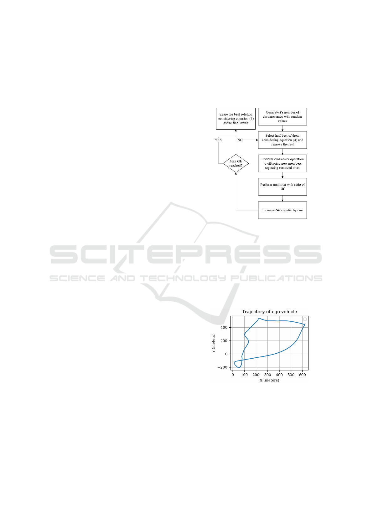
ation step in details. Figure 1 summarizes the genetic

population evaluation cycle.

Figure 1: GA solver to estimate V

and δ.

3 RESULTS AND VALIDATION

DISCUSSION

To validate the formulation and GA solver, one of the

logged data of the e-ATAK automated bus operating

at Stavanger, Norway, is used. Figures 2, 3, and 4 rep-

resent ego vehicles’ trajectory on map frame in me-

ters, heading in rad, and velocity in m/s.

Figure 2: Ego vehicle trajectory from localization.

Table 1 presents parameters with constant values

selected experimentally to present here. Results for

different values of P

and GE are presented to study

the GA solver performance in real-time considering

experiment hardware conﬁguration. Table 2 shows

details of the experiment computer for reference. In

real-time operation, increasing P

and GE increases

GA solver computation load resulting in increasing

VEHITS 2025 - 11th International Conference on Vehicle Technology and Intelligent Transport Systems

224

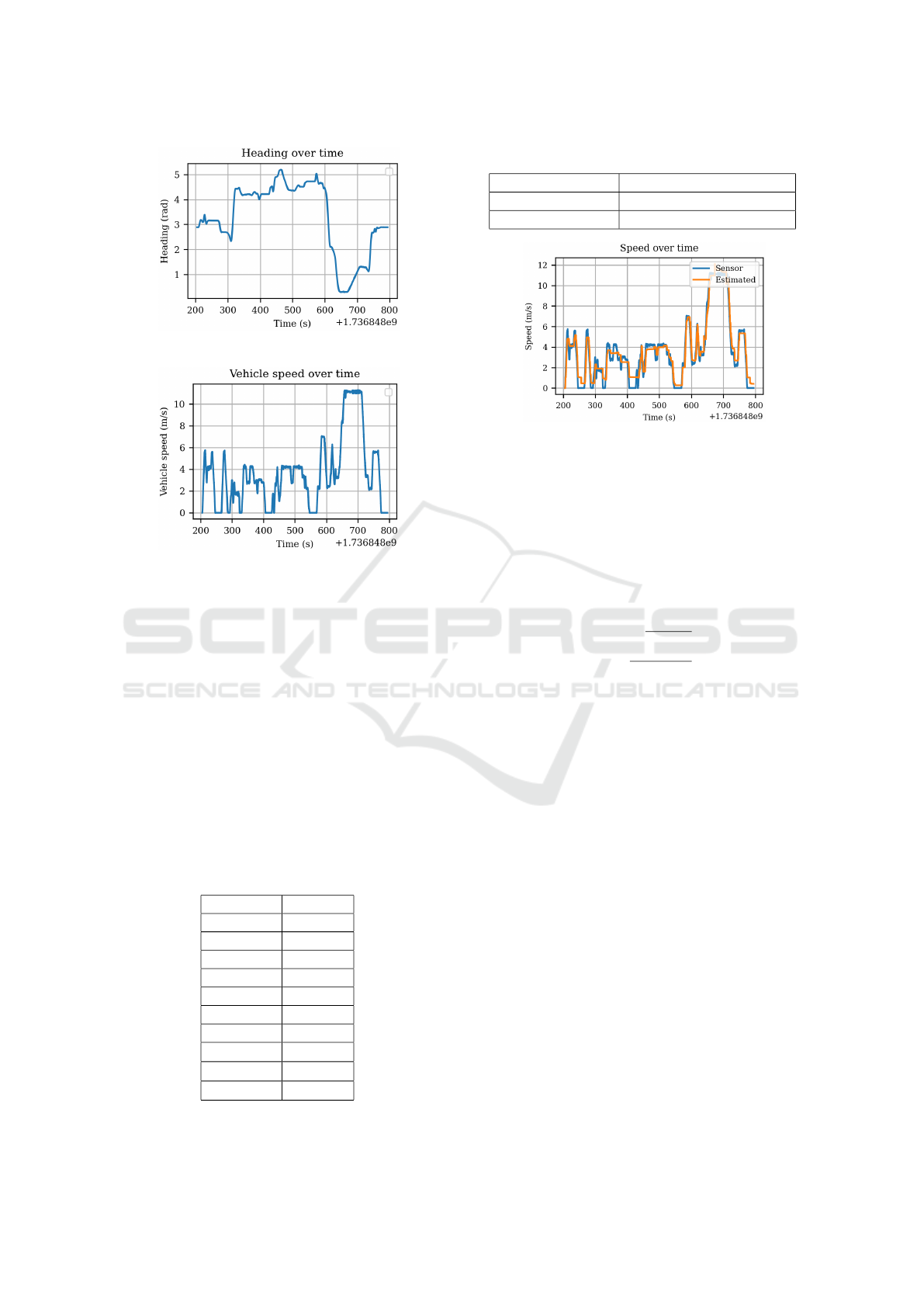
Figure 3: Ego vehicle heading.

Figure 4: Ego vehicle speed.

evaluation execution time. On the other hand, in-

creasing P

and GE will result in better estimation of

the V

, V

and δ

. Figure 5 shows the comparison of

vehicle longitudinal velocity measured from the sen-

sor versus the estimated values where P

= 800 and

GE = 200 as example. Tables 3, 4 and 5 show result

of all experiments with different GE = 100,200, 400

and P

= 400,800, 1200. The success of each conﬁgu-

ration is measured by the calculation of absolute error

of estimated value compared with sensor reading in

the form of error recall at < 0.5m/s, < 1m/s, < 2m/s

and < 5m/s: r@0.5, r@1, r@2 and r@5. Average

Execution Time (AET) for each GE step is also noted

in ms to assess the performance of each conﬁguration

in real-time application.

Table 1: Constant parameters for the present experiment.

Parameter Value

M 0.01

min

-3 m/s

min

-1.5 m/s

min

-0.5 rad

max

18 m/s

max

9 m/s

max

0.5 rad

Table 2: The experiment computer conﬁguration.

Operating System Ubuntu 20.04 LTS

CPU Core i7, 8th Gen, 12-core

RAM 16 GByte DDR4

Figure 5: Ego vehicle estimated speed versus measured

speed from the sensor.

The calculated longitudinal velocity from Dis-

placement Over Time (DOT) is compared with the

proposed method. Displacement over two consecu-

tive localization data obtained as follows:

= X

loc

(t) − X

loc

(t − dt)

= Y

loc

(t) −Y

loc

(t − dt)

(6)

Then, for ego longitudinal velocity:

+ d

(7)

Figure 6 shows the calculated speed using DOT

versus sensor readings. DOT’s highly noisy veloc-

ity estimation can be addressed using low-pass ﬁlters

such as the Moving Average Filter (MAF). The effect

of MAF with different window sizes is also shown,

which indicates improving the speed estimation; how-

ever, low pass ﬁlters such as MAF impose latency on

the measurement. Having 40 Hz localization data, the

time difference between two consecutive location data

will be 25 ms. The latency introduced by MAF with

window size of w will be 25w/2 ms (Smith, 1997).

Table 6 constructed for DOT results with different

MAF windows. Instead of AET, the latency intro-

duced by MAF is indicated to assess real-time appli-

cation performance.

Different approaches could be selected from the

results shown in Tables 3 to 6 considering the prime

objective of this work, to provide redundancy to vehi-

cle speed sensors. This selection will depend on more

details of the ADS module’s ego vehicle speed ac-

curacy requirement from being close enough to real-

time and tolerable deviation from real velocity per-

spectives. For instance, in ADS with a 10 Hz per-

ception rate, latencies and AETs around 100 ms can

Vehicle Longitudinal Speed Estimation Using 3DOF Localization Information and Genetic Solver

225

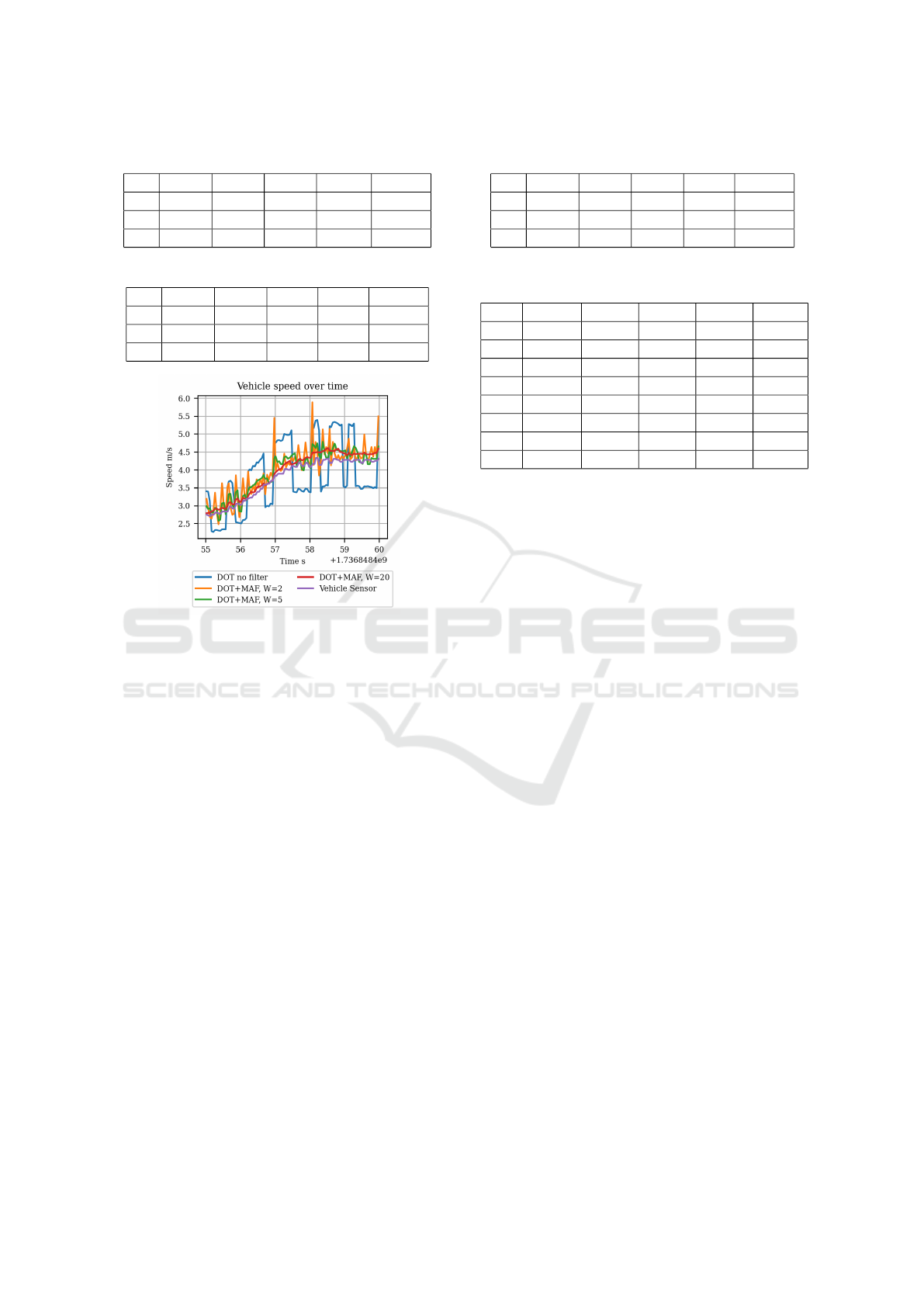
Table 3: The experiment result with P

= 400.

GE r@0.5 r@1 r@2 r@5 AETms

100 4.2% 22.2% 42.7% 84.7% 17.9

200 13.2% 29% 61.1% 100% 32.8

400 51.1% 83% 100% 100% 67

Table 4: The experiment result with P

= 800.

GE r@0.5 r@1 r@2 r@5 AETms

100 19.9% 37% 79% 100% 36.1

200 54.4% 80.1% 100% 100% 66.9

400 98.6% 99.9% 100% 100% 129.6

Figure 6: Ego vehicle calculated velocity using DOT with

different windows size of MAF.

be considered acceptable. Based on this assump-

tion, conﬁgurations at Table 4 with P

= 800 and

GE = 400, Table 5 with P

= 1200 and GE = 200,

also Table 6, using DOT with window size of 10 can

be good candidates. The best performance belongs

to conﬁguration with P

= 1200 and GE = 400, Ta-

ble 5. The closest DOT accuracy is obtained with

a window size of 20, which has less r@0.5 and the

worst time performance. It is worth mentioning that

the AET highly depends on computing conﬁguration

and can be improved with better hardware and soft-

ware implementation. However, the latency imposed

by MAF when using the DOT method is independent

of computation resources.

4 CONCLUSION

The present work attempts to estimate vehicle lon-

gitudinal speed mainly to mitigate speed sensor fail-

ure cases, especially in the SAE level-4 ADS scope,

which requires ADS to detect failures and perform

fail-over maneuvers. To do so, a redundant veloc-

ity estimation method, which uses 3DOF localiza-

tion data, is proposed. Ego longitudinal velocity is

Table 5: The experiment result with P

= 1200.

GE r@0.5 r@1 r@2 r@5 AETms

100 29.9% 64.3% 97.3% 100% 49.9

200 89.3% 99.9% 100% 100% 102

400 99.2% 100% 100% 100% 201.9

Table 6: DOT raw results and MAF output with different

windows size.

win r@0.5 r@1 r@2 r@5 lat ms

1 38% 74% 93% 100% 0

2 89% 97% 99% 100% 25

5 90% 98% 100% 100% 62.5

10 93% 99% 100% 100% 125

20 92% 100% 100% 100% 250

50 86% 100% 100% 100% 625

100 69% 97% 100% 100% 1250

200 55% 80% 99% 100% 2500

estimated using a GA-based optimizer by solving a

SOOP formulated considering the vehicle dynamic

bicycle model. Different conﬁgurations of initial pop-

ulation and generation evaluation steps resulted in

various performances of the method in real-time op-

eration from execution time and the accuracy of esti-

mation perspective. Estimation accuracy is measured

by comparing it to the e-ATAK automated bus speed

sensor. The DOT-based approach for vehicle longi-

tudinal speed calculation is also presented to discuss

the GA performance better, where the velocity calcu-

lation results improved using MAF. Different MAF

window sizes were practiced, which validated the su-

periority of the proposed method compared to the re-

sults of DOT combined with MAF.

The formulation of the current work does not con-

sider the accuracy of localization data. However, the

deviation in the localization information can be in-

cluded in formulating the objective function. Also,

the present work does not study different implemen-

tations and conﬁgurations of cross-over and mutation

operations. The effect of varying hardware conﬁgu-

rations on the proposed method’s performance is also

not addressed in this work. All mentioned topics can

be an extension of the present work. Adding other

measurements next to 3DOF localization information

and using other vehicle dynamic models in problem

formulation can also be different extensions of this

work.

ACKNOWLEDGEMENTS

This work results from collaborative effort and pas-

sion within the ADASTEC Corp. family.

VEHITS 2025 - 11th International Conference on Vehicle Technology and Intelligent Transport Systems

226

REFERENCES

Cassel, A., Bergenhem, C., Christensen, O. M., Heyn, H.-

M., Leadersson-Olsson, S., Majdandzic, M., Sun, P.,

Thors

en, A., and Trygvesson, J. (2020). On percep-

tion safety requirements and multi sensor systems for

automated driving systems. SAE International Jour-

nal of Advances and Current Practices in Mobility,

2(2020-01-0101):3035–3043.

Clavijo, M., Jim

enez, F., Serradilla, F., and D

ıaz-

Alvarez,

A. (2022). Assessment of cnn-based models for

odometry estimation methods with lidar. Mathemat-

ics, 10(18):3234.

Fazekas, M., G

asp

ar, P., and N

emeth, B. (2020). Identiﬁca-

tion of kinematic vehicle model parameters for local-

ization purposes. In 2020 IEEE International Confer-

ence on Multisensor Fusion and Integration for Intel-

ligent Systems (MFI), pages 373–380. IEEE.

Goelles, T., Schlager, B., and Muckenhuber, S. (2020).

Fault detection, isolation, identiﬁcation and recovery

(fdiir) methods for automotive perception sensors in-

cluding a detailed literature survey for lidar. Sensors,

20(13):3662.

Hsu, L.-Y. and Chen, T.-L. (2012). Vehicle dynamic predic-

tion systems with on-line identiﬁcation of vehicle pa-

rameters and road conditions. Sensors, 12(11):15778–

15800.

Jin, X., Yin, G., and Chen, N. (2019). Advanced estima-

tion techniques for vehicle system dynamic state: A

survey. Sensors, 19(19):4289.

Katoch, S., Chauhan, S. S., and Kumar, V. (2021). A re-

view on genetic algorithm: past, present, and future.

Multimedia tools and applications, 80:8091–8126.

Khan, N. H. and Adnan, A. (2017). Ego-motion estimation

concepts, algorithms and challenges: an overview.

Multimedia Tools and Applications, 76:16581–16603.

Kwon, W., Lee, H., Kim, A., and Yi, K. (2025). Lidar-based

odometry estimation using wheel speed and vehicle

model for autonomous buses. International Journal

of Control, Automation, and Systems, 23(1):41–54.

Matos, F., Bernardino, J., Dur

aes, J., and Cunha, J. (2024).

A survey on sensor failures in autonomous vehicles:

Challenges and solutions. Sensors, 24(16):5108.

Par, K., Peker, A. U., Ghahremaninejad, R.,

Ozcan, A., and

Sahin, E. (2024). Introducing ﬂowride® logger, an on-

board data collection framework for commercial auto-

mated vehicles. In VEHITS, pages 488–495.

Pillai, S. and Leonard, J. J. (2017). Towards visual ego-

motion learning in robots. In 2017 IEEE/RSJ Interna-

tional Conference on Intelligent Robots and Systems

(IROS), pages 5533–5540. IEEE.

Saadeddin, K., Abdel-Hafez, M. F., and Jarrah, M. A.

(2014). Estimating vehicle state by gps/imu fusion

with vehicle dynamics. Journal of Intelligent &

Robotic Systems, 74:147–172.

Safavi, S., Safavi, M. A., Hamid, H., and Fallah, S. (2021).

Multi-sensor fault detection, identiﬁcation, isolation

and health forecasting for autonomous vehicles. Sen-

sors, 21(7):2547.

Smith, S. W. (1997). The scientist and engineer’s guide to

digital signal processing. California Technical Pub.

Wang, Y., Mangnus, J., Kosti

c, D., Nijmeijer, H., and

Jansen, S. T. (2011). Vehicle state estimation using

GPS/IMU integration. IEEE.

Wu, M., Lam, S.-K., and Srikanthan, T. (2017). A frame-

work for fast and robust visual odometry. IEEE

Transactions on Intelligent Transportation Systems,

18(12):3433–3448.

Vehicle Longitudinal Speed Estimation Using 3DOF Localization Information and Genetic Solver

227