Efﬁcient Hit-Spectrum-Guided Fast Gradient Sign Method: An

Adjustable Approach with Memory and Runtime Optimizations

Daniel Rashedi

and Sibylle Schupp

Institute for Software Systems, Hamburg University of Technology, Germany

Keywords:

Fault Localization, Neural Networks, Adversarial Input Generation.

Abstract:

Fast Gradient Sign Method (FGSM) is an effective method for generating adversarial inputs for neural net-

works, but it is memory-intensive. DeepFault reduces the memory costs of FGSM by transferring Spectrum-

Based Fault Localization to neural networks. SBFL is a technique traditionally using the execution trace of

a program to identify suspicious code locations that are likely to contain faults. DeepFault employs SBFL to

identify neurons in a neural network that are likely to be responsible for misclassiﬁcations to guide FGSM. We

propose an adjustable hit-spectrum-guided FGSM approach applying a sub-model strategy to avoid gradient

ascent evaluation over the entire model. Additionally, we alter DeepFault’s hit-spectrum computation to be

vector-based to allow parallelization of computation, and we modify the hit spectrum to depend on a speciﬁc

class to allow targeted adversarial input generation. We conduct an experimental evaluation on image clas-

siﬁcation models showing how our approach allows trading off effectiveness of adversarial input generation

with reduced runtimes while maintaining scalability regarding larger models, with maximum runtimes on the

order of tens of seconds. For larger sample sizes, our approach reduces runtimes to fractions of 1/300 and less

compared to DeepFault. When processing larger models, it requires only one-third of FGSM’s memory usage.

1 INTRODUCTION

Fault localization in neural networks gains impor-

tance as research continuously expands deployment

of these systems across diverse domains. Inspired

by traditional software fault localization methods, re-

search has adapted fault localization techniques for

use in neural networks. These methods detect model

design ﬂaws and training issues that negatively impact

a model’s accuracy. A closely related ﬁeld focuses

on adversarial input generation, which reveals model

vulnerabilities through systematically crafted inputs.

The Fast Gradient Sign Method (FGSM) (Good-

fellow et al., 2015) is an approach that generates ad-

versarial input for a model by conducting the gradient

ascent method on a model’s input with respect to its

loss function. That is, FGSM leverages the loss func-

tion as an objective function to maximize in order to

obtain gradients that are used to alter images such that

they are misclassiﬁed by the model. Although FGSM

is efﬁcient in terms of computational runtime, it re-

quires substantial memory overhead.

The DeepFault approach (Eniser et al., 2019)

https://orcid.org/0009-0007-1607-9947

overcomes FGSM’s memory overhead by interpreting

adversarial input generation as a problem of fault lo-

calization in neural networks. Spectrum-Based Fault

Localization (SBFL) (Jones et al., 2002) is a fault

localization technique that traditionally uses execu-

tion traces of software code and outcomes of pass-

ing and failing test cases to identify suspicious code

locations that are likely to contain faults. The out-

come of the test cases contributes to the hit spectrum

of each code location, which is then used to compute

a suspiciousness value. While SBFL was originally

applied to software code, DeepFault transfers SBFL

to neural networks for fault identiﬁcation by consid-

ering correct and incorrect classiﬁcations instead of

test cases. DeepFault applies the outcome of neuron

suspiciousness computation to obtain a list of neurons

considered especially suspicious that serve to guide

FGSM. The approach aims to maximize the output of

suspicious neurons, and thus their impact on the out-

come, to generate adversarial inputs. Although this

approach successfully reduces memory requirements

compared to standard FGSM, it does so at the cost of

increased computational runtime. Our work builds on

the DeepFault approach and aims to enhance memory

and runtime efﬁciency, while also expanding its capa-

Rashedi, D. and Schupp, S.

Efﬁcient Hit-Spectrum-Guided Fast Gradient Sign Method: An Adjustable Approach with Memory and Runtime Optimizations.

DOI: 10.5220/0013463100003964

In Proceedings of the 20th International Conference on Software Technologies (ICSOFT 2025), pages 51-62

ISBN: 978-989-758-757-3; ISSN: 2184-2833

bilities by enabling targeted adversarial input genera-

tion.

Efﬁciency of fault localization methods has been

addressed by several works (Besz

edes, 2019; Zheng

et al., 2016; Wong et al., 2012; Ghosh et al., 2023),

but few fault localization methods for neural networks

report applying modiﬁcations for runtime or memory

optimizations. These types of optimizations are par-

ticularly interesting given the scale of modern neural

networks. Considering both the memory overhead of

FGSM and the computational runtime of DeepFault,

our work aims to enhance the efﬁciency of adversarial

input generation by enhancing DeepFault as follows.

First, we contribute an adjustable sub-model strat-

egy for the adversarial input generation that avoids

exhaustive model analysis. Instead of analyzing all

neurons of a model for their hit-spectra, our approach

creates a sub-model that shares inner layers up to a

speciﬁed layer with the original model. Consequently,

the expensive gradient ascent method is no longer ap-

plied on the entire model but only on the sub-model.

Our experimental evaluation on a MobileNet-V3

and on the SqueezeNet model architecture shows that

our approach allows trading off between adversar-

ial input quality and computational runtime. On the

MobileNet-V3 model, we tested different sub-model

sizes. These led to classiﬁcations of non-target classes

in favor of a target class with ratios of 6.70% and

60.22%, respectively. The smaller and larger sub-

models considered only 464 and 925,856 parameters,

respectively. The observed runtimes were 12.32s and

28.50s for the two sub-models. On the SqueezeNet,

the improvement was less pronounced with a jump

from 6.25% to 22.90% in favor of the target class re-

quiring 22.31s and 30.25s with sub-models of 1792

and 558,144 parameters, respectively.

We conducted experiments on two different mod-

els based on the dense layer model architecture. For

generating 9000 adversarial inputs, our approach re-

quires 1.06s and 1.25s. In comparison, an updated

variant of DeepFault requires 322.24s and 494.94s,

while FGSM requires 1.68s and 1.77s, respectively.

However, for small numbers of adversarial inputs,

our implementation reveals ﬁxed computational over-

head. For generating 100 samples, our approach re-

quires 1.00s and 1.16s on the same models. In com-

parison, the updated variant of DeepFault requires

3.53s and 5.59s, while FGSM requires 0.02s and

0.02s, respectively.

Second, we contribute a vector-based hit-

spectrum computation that replaces DeepFault’s se-

quential neuron hit-spectrum analysis. Our approach

considers only the output layer of the selected sub-

model for hit-spectrum computation compared to

DeepFault that considers all neurons of the original

model. Additionally, we consider the use of vectors

essential to signiﬁcantly improve hit-spectrum com-

putation times as these vectors can be represented

by tensors as provided by modern machine learn-

ing libraries and can thus be computed in a paral-

lelized fashion. On two different models based on

the dense layer model architecture, our implementa-

tion requires 0.26s and 0.25s for hit-spectrum com-

putation on the sub-model, while DeepFault requires

3.72s and 27.09s for the entire original models.

Finally, we extend DeepFault with targeted ad-

versarial capabilities. Unlike the original approach

which only aims to reduce overall accuracy, our

method can guide misclassiﬁcations toward speciﬁc

target classes. We do so by making hit-spectrum com-

putation class-dependent and consider only correct

and incorrect classiﬁcations in favor of a target class.

In summary, our work enhances the DeepFault ap-

proach in three key directions:

1. an adjustable sub-model strategy for input gener-

ation,

2. vector-based hit-spectrum computation, and

3. targeted adversarial input generation capabilities.

To support both reproducibility and further research,

we provide our implementation and evaluation scripts

publicly available on GitHub.

The remainder of this paper is structured as fol-

lows. Section 2 provides an overview of related work.

Section 3 describes the necessary background infor-

mation. Section 4 presents our approach. Section 5

evaluates our approach. Section 6 gives a conclusion.

2 RELATED WORK

Numerous works have already contributed to the do-

main of fault localization in the context of software

code; however, few works have applied this concept

to neural networks. This section covers related works

in the domain of fault localization for neural networks

and compares their contributions to our work’s contri-

bution.

DeepFault’s approach (Eniser et al., 2019) serves

as a foundation for this work as it is the ﬁrst to

transfer the concept of spectrum-based fault local-

ization to neural networks. Other works have also

contributed improvements to DeepFault. (Hashemi-

far et al., 2024) improves the DeepFault approach by

expanding suspiciousness computation from individ-

ual neurons to pathways of neurons. The approach

https://github.com/IDahera/

fast-hs-adversarial-input-gen.git

ICSOFT 2025 - 20th International Conference on Software Technologies

presented in (Duran et al., 2021), a variant of Deep-

Fault, increases the original approach’s granularity by

not only considering a model misclassifying any sam-

ple of a selected class, but also considering pairs of

source and target classes. Our work addresses the us-

age of spectrum-based fault localization in neural net-

works, and it aims to improve its memory and runtime

performance. To the best of our knowledge, the works

improving DeepFault’s approach focus on improving

the quality of fault localization rather than addressing

memory or runtime efﬁciency optimizations.

Besides SBFL, Mutation-Based Fault Localiza-

tion (MBFL) approaches have also been transferred to

neural networks in aiding model development. Deep-

MuFL (Ghanbari et al., 2024) introduces a novel

approach to fault localization in neural networks

through mutation-based methods. DeepMuFL sys-

tematically modiﬁes the network to guide developers

in identifying and addressing design problems. Yin

et al. propose DFauLo (Yin et al., 2023), an ap-

proach that generates mutants by training copies of

a given model on strategically selected training sam-

ples. The behavior of these mutants on selected sam-

ples is compared to the behavior of the original model

to derive a likelihood for speciﬁc samples containing

faults. However, to the best of our knowledge, none

of the MBFL works report optimizing fault localiza-

tion methods for neural networks in terms of memory

or runtime efﬁciency.

Recent research in the domain of fault localiza-

tion for neural networks has also proposed a series of

methods (Wardat et al., 2022; Eniser et al., 2019; Cao

et al., 2022; Usman et al., 2021) applying static and

dynamic approaches on neural networks to identify is-

sues in their design or training process. Static checks

apply patterns of best practices in model initialization

and compilation to avoid executing models. Dynamic

approaches, on the other hand, gather traces of model

execution such as parameter valuations or classiﬁca-

tion outcomes to identify and locate problems such as

model design issues or improvable selection of train-

ing parameters. Neither of these works addresses tra-

ditional fault localization methods or improvement of

their memory and runtime efﬁciency.

3 BACKGROUND

This section brieﬂy covers the concept of SBFL and

its application to neural networks as proposed by the

work (Eniser et al., 2019). As described in prior

sections, SBFL is a method from software fault lo-

calization that traditionally uses execution traces of

software code in combination with positive and neg-

ative test outcomes to identify code regions statisti-

cally more likely to contain faults. Intuitively, the hit

spectrum of a code region is determined by two fac-

tors: ﬁrst, whether a line of code was executed (hit)

or not executed (miss), and second, whether the corre-

sponding test case passed or failed. The combination

of these factors determines the statistical likelihood of

a fault in that code region. The hit spectrum is then

used to compute a suspiciousness value for each code

region. The following deﬁnitions show how the con-

cept of SBFL is transferred to neural networks as a

basis for the remainder of this work.

Deﬁnition 3.1 (Neural Network). We deﬁne a neural

network as a 3-tuple M = (N,E,L) where N is a set

of neurons, E is a set of edges, and L = {l

,... , l

}

is a set of k layers with ∀i, j ∈ {1,... , k} : l

⊂ N and

∩ l

0 if i ̸= j. We consider each neuron φ ∈ N to

represent an activation function φ : R

→ R mapping

m-dimensional real values to a single real value.

The deﬁnition of a neural network serves as a basis

to deﬁne the hit spectrum of a neuron in the following.

Without loss of generality, we can assume that layer

is the input layer and layer l

is the output layer of

the neural network M . This assumption is valid as

we can relabel the layers accordingly. Furthermore,

we can also construct layers consisting of only one

neuron to cover various model designs.

Deﬁnition 3.2 (Hit Spectrum of a Neuron (Eniser

et al., 2019)). Given a neural network M = (N, E,L)

with a set X = {x

,... , x

} of input samples for M ,

the hit spectrum of a neuron φ ∈ N is deﬁned as the

4-tuple HS

(φ) = (a

) as follows:

• a

∈ N is the number of samples x

∈ X that acti-

vate φ and are correctly classiﬁed by the model.

• a

∈ N is the number of samples x

∈ X that acti-

vate φ and are misclassiﬁed by the model.

• n

∈ N is the number of samples x

∈ X that do

not activate φ and are correctly classiﬁed by the

model.

• n

∈ N is the number of samples x

∈ X that do

not activate φ and are misclassiﬁed by the model.

A sample x ∈ R

activates a neuron φ if φ(x) > δ.

However, in practice, neurons from any layer other

than the input layer receive their input from other neu-

rons. In Section 5, we conducted our experiments

with a threshold of δ = 0 for the models used, as

this value already leads to reasonable suspiciousness

value distributions among the selected layers’ neu-

rons. We expect that higher values of δ may serve

useful if the selected activation function in combina-

tion with the model’s input samples lead to overall

high activation ratios in the model’s layers. Also note

Efﬁcient Hit-Spectrum-Guided Fast Gradient Sign Method: An Adjustable Approach with Memory and Runtime Optimizations

that for simpliﬁcation purposes, our above notation

does not explicitly represent weights or biases in the

activation function φ. Although the weights and bi-

ases are present in real-world neural networks, they

are not signiﬁcant for the workﬂow of our approach

as described in following sections.

The neuron hit spectrum is then used to compute a

suspiciousness value for each neuron φ ∈ N using one

of multiple well-known suspiciousness functions. We

have selected two standard metrics that the reference

work (Eniser et al., 2019) also makes use of, namely

Tarantula (Jones et al., 2002) and Ochiai (Abreu et al.,

2006), to compute the suspiciousness value of a neu-

ron. Both metrics compute a ratio based on the hit

spectrum of the given neuron.

Tarantula(a

) =

(1)

In Tarantula, the numerator term captures the ratio of

failed test cases upon activation of the neuron to the

total number of failed test cases. Accordingly, the sec-

ond addend of the denominator term captures the ratio

of passed test cases upon activation of the neuron to

the total number of passed test cases. Tarantula com-

pares the former fraction to the sum of both fractions

to compute the suspiciousness value of a neuron.

Ochiai(a

) =

+ n

) · (a

+ a

)

(2)

In comparison, the Ochiai metric calculates suspi-

ciousness using the ratio of failed test cases where

the neuron is activated (a

in the numerator) to the

square root of two terms multiplied together in the

denominator: (a

+ n

) representing the total num-

ber of failed test cases regardless of neuron activation,

and (a

+ a

) representing the total number of times

the neuron was activated across both passed and failed

test cases.

4 APPROACH

Our work enhances the DeepFault approach (Eniser

et al., 2019) by addressing the approach’s memory

and runtime efﬁciency, while also expanding its capa-

bilities from general to targeted adversarial input gen-

eration. First, we describe our hit-spectrum computa-

tion in terms of vector arithmetic for usage of modern

tensor libraries. These libraries allow reducing time

complexity as they use parallelized tensor arithmetic

computation. Additionally, we provide a modiﬁca-

tion that computes the hit spectrum with respect to a

target class to obtain suspiciousness values for neu-

rons that guide towards misclassiﬁcation in favor of

the selected class. This modiﬁcation contributes to

the generation of targeted adversarial inputs. Second,

we propose a gradient ascent method that leverages a

sub-model strategy for input synthesis.

4.1 Targeted Hit-Spectrum

Computation

One of our approach’s key components is an updated

hit-spectrum computation method that leverages vec-

tor arithmetic to improve runtimes. Algorithm 1 de-

picts our proposed approach. The algorithm iterates

over the samples X

= {x

,... , x

} of target class t

and computes the hit spectrum of layer l

as follows.

First, model M is evaluated on the provided sample

and the approach initializes variables y and α con-

taining the output of the model for this sample and

the corresponding activation values of layer l

, respec-

tively. Next, we obtain vectors a

, a

, n

, and n

using

logical conjunction and negation operations to con-

struct the layer’s hit spectrum. We assume that y and

are binary vectors for element-wise equality to ob-

tain h deﬁned by =

. Given two m-dimensional vec-

tors a and b, we assume that for c = (a =

b) the fol-

lowing holds.

∀i ∈ {1, ..., n} : c

(

1 if a

= b

0 if a

̸= b

(3)

In practice, the binary vectors are manually obtained

by making only the element of y contain value 1 at the

index that model M predicts as the output class, α

contains 1 at an index if a threshold activation value

for the corresponding neuron is reached. In the same

manner, we assume vectors h and α to be binary vec-

tors. Finally, the binary vectors h and α must be con-

verted to integer vectors. This allows performing the

sum operation in the next step to adjust the currently

computed hit spectrum of the layer. The process is

repeated for all selected samples.

Note that we have chosen to use only samples X

of class t to compute the hit spectrum of layer l

in-

stead of using the entire set of available samples. Es-

sentially, we conduct hit-spectrum computation with

respect to samples of a target class t that the approach

generates adversarial samples for. By doing so, the hit

spectrum derived from this reduced sample set intu-

itively no longer captures the suspiciousness for gen-

eral misclassiﬁcations, but it captures suspiciousness

for misclassiﬁcations in favor of class t. Of course,

one may also consider samples of arbitrary classes if

regular adversarial input generation is the goal. Also

note that our approach only considers the output layer

of the sub-model for hit-spectrum computation. This

ICSOFT 2025 - 20th International Conference on Software Technologies

Input: model M , layer l

, sample set X

and

set Y

= {y

,... , y

} of expected

outputs

Result: hit spectrum hs

of layer l

over X

) ← (0, 0,0,0);

for x

∈ X

(y,α ← (M .out put(x

),l

.active(x

));

h ← (y =

) [hit vector];

← a

+ h ∧ α;

← a

+ ¬h ∧ α;

← n

+ h ∧ ¬α;

← n

+ ¬h ∧ ¬α;

end

return hs

= (a

)

Algorithm 1: Targeted Hit-Spectrum Analysis Us-

ing Vector Arithmetic.

is a contrast to the original DeepFault approach that

computes hit spectrums for all neurons.

By leveraging vector arithmetic our approach for

hit-spectrum computation becomes runtime efﬁcient

and scalable for modern hardware and modern li-

braries such as TensorFlow or PyTorch conducting

parallelized vector and matrix computation. The al-

ternative as conducted by related work (Eniser et al.,

2019) iterates over neurons in a layer using scalar

operations. Time complexity for our computation of

can be estimated by

Time complexity: O(n/p) (4)

where n is the number of neurons in layer l

and p

is the number of processing units. A linear approach

would have a time complexity of O(n) as it requires

considering individual scalar operations.

In contrast to time complexity, our modiﬁcations

raise the space complexity. Instead of storing scalar

values, entire vectors of length n are stored leading to

the following space complexity

Space complexity: O(3n) = O(n) (5)

as both input vectors of each operation and the out-

come must be stored in memory during parallelized

computation.

4.2 Gradient Ascent Method

Leveraging Sub-Model Strategy

Next, we describe our approach for generating adver-

sarial inputs using a gradient ascent method applying

a sub-model strategy. Neural networks with larger

neuron numbers can pose signiﬁcant computational

challenges with their regular forward pass. Applying

the chain rule for backpropagation in the context of

gradient ascent ampliﬁes the computational demands

on time and space requirements. For that reason, we

propose a sub-model strategy that no longer conducts

backpropagation on the entire model but only on the

layers of the sub-model to obtain a fraction of the pre-

vious time and space requirements.

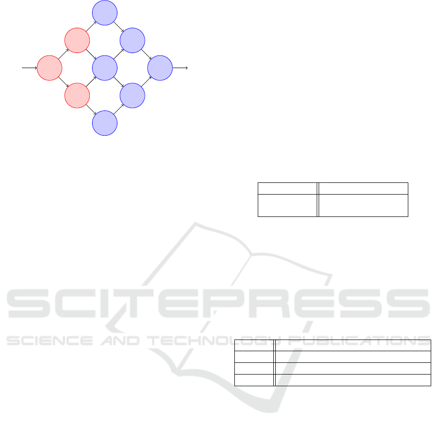
Figure 1 illustrates one example of how to ob-

tain a sub-model from a given model. In this model,

we have colored neurons in red to indicate the sub-

model’s neurons such that only 3 out of 9 neurons

are considered for the gradient ascent method. Please

note that the sub-model strategy is not limited to se-

quential models, but can be applied to any model ar-

chitecture. Section 5 covers our experimental evalua-

tion which also considers non-sequential models. We

have chosen to manually select layer conﬁgurations

to obtain sub-models for the selected non-sequential

models as an automated sub-model generation ex-

ceeds the scope of this work.

Input: model M

′

, hit spectrum hs

of layer

, suspiciousness function

σ ∈ {Tarantula, Ochiai}, sample

set X

to modify

Result: modiﬁed sample set X

′

← σ(hs

) ;

Ω ← top

sus indices(s

,k) ;

′

← X ;

for t ∈ iterations do

′

← RunModel(M

′

) ;

∇ ←

∂(

∑

i∈Ω

′

[i])

∂X

′

;

′

← X

′

+ ∇ ∗ ε

end

Algorithm 2: Adversarial Input Generation Using

Sub-Model Strategy.

Algorithm 2 describes our approach. Considering

some model M = (N, E, L), the algorithm takes as

input

• a set of samples X

not of the target class t,

• the computed hit spectrum hs

for layer l

• σ ∈ {Tarantula, Ochiai} as the suspiciousness

function,

• sub-model M

′

= (N

′

) where N

′

⊂ N, E

′

⊂

E such that ∀e ∈ E

′

: e = (n

pre

post

) it holds

pre

post

∈ N

′

, and L

′

⊂ L such that ∀l

∈ L

′

holds l

⊂ N

′

Note that the main algorithm does not need to con-

sider any target class because targeted hit-spectrum

computation is conducted in the prior step.

During initialization, the algorithm computes the

layer’s suspiciousness values using the provided sus-

Efﬁcient Hit-Spectrum-Guided Fast Gradient Sign Method: An Adjustable Approach with Memory and Runtime Optimizations

1,1

2,1

2,2

3,1

3,2

3,3

4,1

4,2

5,1

Figure 1: Example of a sub-model.

piciousness metric σ. Then, it determines the k neu-

rons with the largest suspiciousness values. Note that

the k most suspicious neurons we consider are all in-

cluded in the sub-model’s output layer. Section 5 cov-

ers our experimental evaluation of the algorithm and

gives insight on appropriate values for these parame-

ters. Additionally, the algorithm creates a copy X

′

the samples to be modiﬁed.

Based on the approach DeepFault (Eniser et al.,

2019), the algorithm’s loop ﬁrst conducts a forward

pass on the samples to be modiﬁed by executing the

model via RunModel to obtain the sub-model’s out-

put. Then, it computes the gradient ∇ by taking the

partial derivative of the sub-model’s most suspicious

neurons’ output with respect to the current version

of the samples. Recall that the layer l

is the output

layer of the sub-model and contains the most suspi-

cious neurons. Finally, the main step of the algorithm

updates the samples X

′

by adding the gradient multi-

plied by some value ε. These steps are repeated for a

predeﬁned number of iterations.

5 EVALUATION

This section is dedicated to the experimental evalua-

tion of our proposed approach. After providing details

on the system setup, we describe the research ques-

tions and associated experiments. As part of the ﬁrst

research question, we investigate our approach’s sub-

model strategy. Speciﬁcally, we examine how it al-

lows trading off runtimes and memory usage for qual-

ity of adversarial input generation. We do so by com-

paring different sub-model conﬁgurations for two se-

lected public models trained on the public cifar10

dataset. As part of the second research question, we

compare efﬁciency of our approach against the re-

lated work, DeepFault, and the original FGSM at-

tack. Finally, we evaluate how various parameters im-

pact both quality of adversarial input generation and

runtime efﬁciency, identifying conﬁgurations that im-

prove results while maintaining short execution times.

Before proceeding with the research questions and

their evaluation, we provide details on the software

and hardware speciﬁcations to ensure experimental

reproducibility. For our experiments, we have cho-

sen to implement our approach in Python using the

PyTorch (torch) library and the torchvision li-

brary for creating instances of publicly available im-

age classiﬁcation models. For both libraries, we have

used the recent stable versions available at the time

of conducting the experiments. Table 1 provides de-

tails on the software speciﬁcation used for our exper-

iments.

Table 1: Software Speciﬁcations.

OS ubuntu@22.04

Python 3.12 torch@2.4.0

torchvision@0.19.0

We conducted experimental evaluation on a sys-

tem with a hardware speciﬁcation given in Table 2.

Note that although the system has two GPUs, our

implementation was not adapted to split computation

across multiple GPUs. Early attempts to enable Py-

Torch’s built-in multi-GPU support indicated the need

for sophisticated modiﬁcations beyond the scope of

this work.

Table 2: Hardware Speciﬁcations.

CPU AMD Ryzen 2990WX 32-Core CPU

GPU 1 RTX 2080 Ti (11.264 MiB)

GPU 2 RTX 2080 Ti (11.264 MiB)

RAM 125 GiB

For our experiments, we have chosen to evaluate

our approach on 4 models and 3 datasets. We chose

two simpler models, a small dense layer model and

a small convolutional layer model based on LeNet

(LeCun et al., 1998), which we trained and evalu-

ated on the mnist and fashion mnist (abbreviated

as f-mnist in tables) datasets to cover simpler sce-

narios. Additionally, we also used the MobileNet V3

Small (MNV3) (Howard et al., 2019) and SqueezeNet

(SN) (Iandola et al., 2016) models trained on the

cifar10 dataset to evaluate our approach on larger

and more complex models and datasets to cover sce-

narios closer to an actual application. During initial-

ization, every model was trained for 5 epochs on the

corresponding training set using the Adam optimizer

(Kingma and Ba, 2014). Table 3 gives an overview

of the models, the associated datasets, the number of

parameters, and the accuracy of the models on the cor-

responding test set.

ICSOFT 2025 - 20th International Conference on Software Technologies

Table 3: The models and the associated datasets used for

evaluation.

Model Dataset Parameters Acc.

LeNet mnist 28,534 98.63 %

DenseNet mnist 576,810 97.28 %

LeNet f-mnist 28,534 88.65 %

DenseNet f-mnist 576,810 87.42 %

MNV3 cifar10 2,542,856 87.74 %

SN cifar10 1,235,496 79.00 %

5.1 RQ1: Trading off Runtimes and

Memory Usage for Adversarial

Input Generation Quality

As part of the ﬁrst research question, we investi-

gate how our sub-model strategy enables trading off

between runtime performance, memory usage, and

adversarial input generation quality. We conducted

these experiments exclusively on the MNV3 and SN

models trained on the cifar10 dataset as we expect

minor differences in different conﬁgurations of sub-

models for the smaller scale models with much fewer

neurons and layers. For each model, we constructed

two different conﬁgurations of sub-models, one with

a sub-model containing less than 1 percent of the orig-

inal model’s neurons and one with layers containing

roughly 30 to 45 percent of the original model’s neu-

rons. Table 4 provides an overview of the sub-model

conﬁgurations used for evaluation. We have selected

the following parameters for the experiments:

• |X| = 9000: number of non-class-0 samples to be

modiﬁed,

• k = 5: number of most suspicious neurons se-

lected,

• iterations = 5: iterations for the modiﬁcation pro-

cess,

• σ = Ochiai, and

• ε = 1.0: gradient factor.

Table 4: The sub-model conﬁgurations.

Model Parameters Size Ratio

MNV3 (A) 464 0.02 %

MNV3 (B) 925,856 36.41 %

SN (C) 1,792 0.15 %

SN (D) 558,144 41.18 %

Table 5 provides an overview of the results of the

experiments conducted for RQ1. The table shows the

resulting percentage of predictions in favor of the tar-

get class and the corresponding durations for the ad-

versarial input generation process. The results show

that the percentage of predictions in favor of target

class t = 0 signiﬁcantly increases with the number of

parameters of the sub-model. This is expected as the

sub-models with more parameters are able to capture

more of the original model’s behavior. However, the

results also show that the duration of the adversar-

ial input generation process increases with the num-

ber of parameters of the sub-model. These results

demonstrate how our approach allows for a trade-off

between the percentage of predictions in favor of the

target class and the duration of the adversarial input

generation process. Our key ﬁndings include:

• Our approach was capable of modifying the sam-

ples such that the original model misclassiﬁed

6.7% in favor of target class t = 0 although sub-

model A itself contains 0.02% of the original

model’s parameters.

• By increasing runtimes, sub-model B with

36.41% of the original model’s parameters had a

60.22% misclassiﬁcation rate in favor of the target

class.

• We make similar observations on both variants

of the SN model. However, the misclassiﬁcation

rates in favor of class t = 0 are lower compared to

the MNV3 model. This could be due to the SN

model’s lower accuracy on the cifar10 dataset

possibly related to its smaller size. Its speciﬁc ar-

chitecture could also make the selected neurons

less effective for adversarial input generation.

The relationship between sub-model size and process-

ing duration is not strictly linear. We hypothesize that

this non-linearity may be attributed to data transfer

overhead between different memory locations, partic-

ularly when moving datasets and models to and from

GPU memory.

Table 5: Target class prediction rates and runtimes for dif-

ferent sub-model conﬁgurations.

Model t-Pred. Time (s)

MNV3 (A) 6.70 % 12.32

MNV3 (B) 60.22 % 28.50

SN (C) 6.25 % 22.31

SN (D) 22.90 % 30.25

5.2 RQ2: Comparison of Runtimes and

Memory Usage Against FGSM and

DeepFault

Next, we compare our approach’s runtimes and mem-

ory usage against DeepFault and regular FGSM.

More speciﬁcally, we compare:

Efﬁcient Hit-Spectrum-Guided Fast Gradient Sign Method: An Adjustable Approach with Memory and Runtime Optimizations

• hit-spectrum computation runtimes between

DeepFault on complete models and our approach

on sub-models, and

• input synthesis runtimes between all three ap-

proaches.

For the experimental evaluation we used the following

setup consisting of:

• DF@tf1: the publicly available source code of

DeepFault

which uses TensorFlow Version 1

(tensorflow@1.13.2),

• DF@tf2: a custom version of DeepFault that

we have migrated to TensorFlow Version 2

(tensorflow@2.12.00) for a more meaningful

comparison as we are aware of the numerous im-

provements of TensorFlow Version 2 over Version

1, and

• FGSM: a custom version of FGSM we imple-

mented using PyTorch (torch@2.4.0) for our ex-

isting experimental setup initially introduced due

to the original approach being a well-known at-

tack of simpler nature so that we obtain a better

comparison,

Due to the substantial differences between the imple-

mentation of PyTorch and TensorFlow, we avoided a

migration of DeepFault to PyTorch because we con-

sider the required changes. Nonetheless, our experi-

ments use the original DeepFault implementation for

comparison to cover the original authors’ work and

intentions. Note that we also applied minor modiﬁca-

tions to both DeepFault variants to conduct our exper-

iments’ runtime measurements.

First, we examine the hit-spectrum computation

times of DeepFault and our approach. We use two

dense layer models using the reLU function as ac-

tivation function listed in Table 6. Both models

Table 6: Dense layer models used for experimental evalua-

tion.

Model Description

8x20-DenseNet

8 dense layers

each with 20 neurons

10x100-DenseNet

10 dense layers

each with 100 neurons

were trained on the mnist dataset for 5 epochs us-

ing the Adam optimizer. We selected this dense layer

model architecture because it was also used by (Eniser

et al., 2019) for experimental evaluation, and it is na-

tively supported by their implementation without fur-

ther modiﬁcations. Moreover, we chose two different

https://github.com/hfeniser/DeepFault

models to better capture the applications’ behavior on

different model sizes.

Table 7 provides an overview of the determined

hit-spectrum computation times of both DeepFault

versions and our approach. The results show that

our approach is signiﬁcantly faster than both DF@tf1

and DF@tf2 for both models. Our approach takes

0.26s and 0.25s for the 8x20-DenseNet and 10x100-

DenseNet models, respectively. In contrast, DF@tf1

takes 3.72s and 27.09s, and DF@tf2 takes 4.82s and

22.02s for the same models. That is, our approach

computes the hit spectrum for 8x20-DenseNet and

10x100-DenseNet roughly 14 times and 104 times

faster than DF@tf1, respectively, With respect to

DF@tf2, our approach computes the hit spectrum

for 8x20-DenseNet and 10x100-DenseNet roughly 19

times and 88 times faster, respectively. To wrap it

up, implementing the hit-spectrum computation using

tensors leads to a signiﬁcant runtime improvement.

Table 7: Computation times for hit-spectrum generation us-

ing 20 batches each of 64 samples.

Approach DenseNet

8x20 10x100

DF@tf1 3.72 s 27.09 s

DF@tf2 4.82 s 22.02 s

Our Work 0.26 s 0.25 s

Next, we compare the input synthesis times of

DF@tf1, DF@tf2, FGSM, and our approach by con-

ducting the experiments again on the 8x20-DenseNet

and 10x100-DenseNet models. Table 8 and Table 9

provide an overview of the determined input synthe-

sis times of the different approaches instructed to gen-

erate 10,100, 1000, 9000 adversarial samples respec-

tively. We make multiple noteworthy observations.

Our approach reveals small variations with grow-

ing sample sizes. For 100 samples it takes 1.02s for

the 8x20-DenseNet model and 1.16s for the 10x100-

DenseNet model. However, with 9000 samples, the

runtimes are 1.06s and 1.25s for the 8x20-DenseNet

and 10x100-DenseNet models, respectively. The run-

times increase only by 0.06s and 0.09s, respectively.

Our implementation likely has ﬁxed overhead costs

in data processing and memory management. While

these cause higher initial runtimes, their impact be-

comes negligible with larger datasets.

DF@tf1 is not capable of generating adversarial

samples for any of the models with 1000 and 9000

samples within a reasonable time frame. DF@tf1

takes signiﬁcantly longer than the other approaches

with 2020.84s for 100 samples. Additionally, its run-

times appear to increase exponentially. 100 sam-

ples take 2020.84s which far surpasses its runtimes

ICSOFT 2025 - 20th International Conference on Software Technologies

of 7.81s for 10 samples that we measured separately.

That is, repeating the input generation for 10 samples

multiple times appears to be more efﬁcient. We sus-

pect that the larger delays are caused by the imple-

mentation’s usage of the outdated TensorFlow Ver-

sion 1 which may perform non-optimal memory man-

agement leading to memory overhead.

DF@tf2 demonstrates more efﬁcient runtimes

than DF@tf1, with computation times roughly pro-

portional to sample sizes. It ranges from 3.53s on 100

samples to 322.24s on 9000 samples for the 8x20-

DenseNet model, and it ranges from 0.59s on 100

samples to 494.94s on 9000 samples for the 10x100-

DenseNet model. Hence, DF@tf2 requires notably

more time for 100 samples, and signiﬁcantly more

time for 9000 samples.

FGSM has the fastest runtimes for both models

with 10-1000 samples. However, with 9000 samples,

our approach outperforms FGSM - running 0.62s

faster for the 8x20-DenseNet model (1.06s total) and

0.52s faster for the 10x100-DenseNet model (1.25s

total). When generating larger sample sets for the

larger models MNV3 and SN using FGSM, we en-

countered memory overﬂows, prompting further in-

vestigation of memory requirements. This observa-

tion leads to the next experiment.

Table 8: Runtime comparison of selected input synthe-

sis methods on 8x20-DenseNet model with varying sample

sizes.

Approach Number of Samples

100 1000 9000

DF@tf1 2020.84 s N/A N/A

DF@tf2 3.53 s 36.07 s 322.24 s

FGSM 0.02 s 0.19 s 1.68 s

Our Work 1.02 s 1.27 s 1.06 s

Table 9: Runtime comparison of selected input synthesis

methods on 10x100-DenseNet model with varying sample

sizes.

Approach Number of Samples

100 1000 9000

DF@tf1 2993.29 s N/A N/A

DF@tf2 5.59 s 53.33 s 494.94 s

FGSM 0.02 s 0.20 s 1.77 s

Our Work 1.16 s 1.29 s 1.25 s

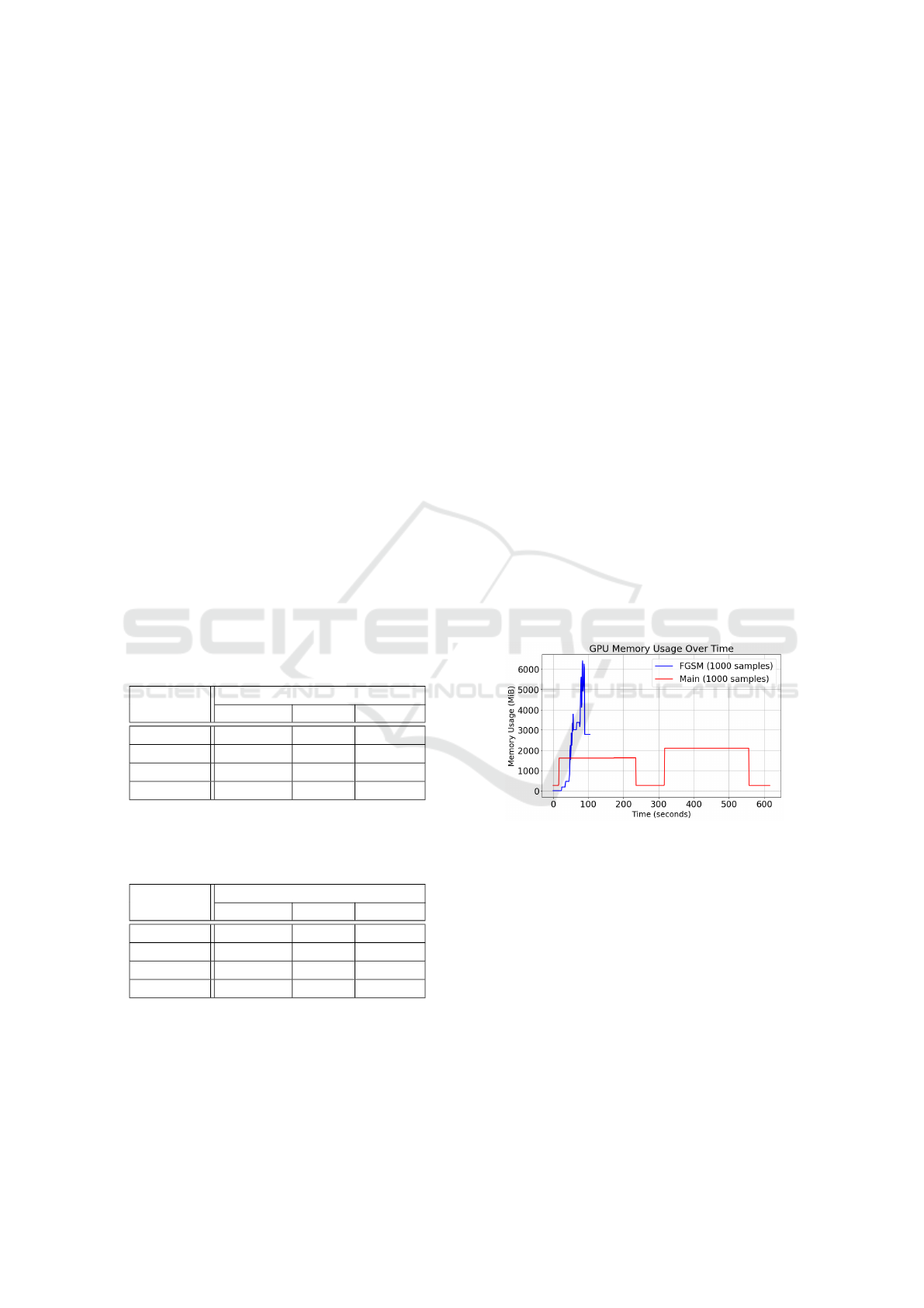
We also conducted experiments to evaluate the

memory usage of our approach and FGSM for gen-

erating adversarial samples. To examine the mem-

ory usages of FGSM and our approach, we have used

the larger model MNV3 and SN as inputs and in-

structed both approaches to generate 1000 adversar-

ial samples. More speciﬁcally, we have measured the

GPU memory usage of both approaches ﬁrst generat-

ing 1000 samples for the MNV3 model and then for

the SN model. Figure 2 provides a graph of the re-

sulting memory usage of both approaches. We make

the following observation: FGSM requires less time

for the synthesis of adversarial samples, but it also re-

quires more memory. More speciﬁcally, it required

roughly 100s as opposed roughly 550s on our ap-

proach for the sequence of both models. However,

for only 1000 samples, FGSM peaks at 6414 MiB, our

approach peaks at 2106 MiB, hence requiring roughly

one-third of memory usage. We consider this to be the

reason for the aforementioned memory overﬂows we

have encountered while attempting to generate 9000

samples immediately using FGSM.

To wrap the evaluation for research question 2 up,

we conclude from the experimental results:

• that our approach is able to outperform both

DeepFault and FGSM in terms of runtimes con-

sidering especially large numbers of samples to

synthesize, and

• our approach slightly falls behind FGSM in terms

of runtimes for smaller sample sizes, but it is able

to generate adversarial samples for larger models

and datasets with signiﬁcantly less memory usage.

Figure 2: GPU memory usage over time comparing our ap-

proach with FGSM in generating 1000 adversarial samples

for the MNV3 and SN models.

5.3 RQ3: Effectiveness of Adjustable

SBFL-guided Target Adversarial

Input Generation

As part of the last research question, we evaluate

the effectiveness of our approach on adversarial input

generation. First, we want to examine whether the

modiﬁcations on hit-spectrum computation and input

synthesis indeed succeed in adversarial input that mis-

classiﬁed in favor of the selected class. Secondly, our

experiments investigate the impact of different param-

eter values on the effectiveness and runtimes of the

Efﬁcient Hit-Spectrum-Guided Fast Gradient Sign Method: An Adjustable Approach with Memory and Runtime Optimizations

adversarial input generation process. We identify the

following list of parameters that we consider relevant

with respect to effectiveness and runtimes of our im-

plementation beyond sub-model conﬁgurations:

• k: the number of most suspicious neurons to be

used for adversarial input generation,

• iterations: the number of iterations for the modi-

ﬁcation process, and

• ε: the gradient factor.

We expect that k is a parameter that affects the effec-

tiveness of the adversarial input generation process,

while iterations and ε are parameters that affect the

runtimes of the adversarial input generation process.

For the third research question, we again con-

sider the previously described models, namely LeNet,

Dense, MNV3, and SN. For all models we have cho-

sen to select a sub-model representing roughly half

the size of the original model. To evaluate the ap-

proach’s effectiveness at generating targeted adversar-

ial inputs, only samples from non-target classes (ex-

cluding class t = 0) were selected for modiﬁcation.

Number of Neurons K. The ﬁrst experiment varies

the number of neurons to become targets for adver-

sarial input generation such that we consider k ∈

{10,50}. Table 10 lists the obtained prediction rates

in favor of the target class and the associated runtimes.

In 4 out of 6 cases, we consider the improvements

in prediction rates to be insigniﬁcant. The DenseNet

model trained on mnist even shows a slight decrease

in prediction rates. At the same time the runtimes ap-

pear to increase roughly by factors of 2-3.5. For in-

stance, the SN model improves from 6.32% to 7.69%

with k = 50, but the runtime also increases from

32.75s to 114.96s. Only the LeNet models trained on

mnist and f-mnist show signiﬁcant improvements

in prediction rates with k = 50. They increase from

0.64% to 24.13% and from 46.13% to 63.34%, re-

spectively. We conclude that the number of neurons

selected for adversarial input generation certainly af-

fects runtimes signiﬁcantly, however, improvements

appear to depend on the model architecture.

Number of Iterations. The number of iterations to

apply the gradient ascent algorithm is the next param-

eter we investigate. We consider it particularly inter-

esting because choosing different numbers of itera-

tions may grant insight into beneﬁts obtained from re-

peating the gradient ascent loop rather than repeating

the whole process. Usage of the loop allows keeping

the models and datasets in memory instead of reload-

ing them. This could serve useful in scenarios where

the optimal number of iterations or gradient factor is

Table 10: Our implementation’s prediction results on class

t = 0 and corresponding runtimes on various models using

varying number of neurons k.

Model k t-Pred. Time (s)

DenseNet

(mnist)

10 63.10% 2.71

50 62.04% 9.33

DenseNet

(f-mnist)

10 63.64% 3.05

50 63.69% 7.15

LeNet

(mnist)

10 0.64% 3.89

50 24.13% 7.15

LeNet

(f-mnist)

10 46.13% 3.78

50 63.34% 9.57

MNV3

(cifar10)

10 6.71% 15.42

50 7.01% 37.01

(cifar10)

10 6.32% 32.75

50 7.69% 114.96

unknown such that the process can be repeated until

convergence of prediction rates.

Table 11 lists the obtained prediction rates in

favor of the target class and the associated run-

times with iterations ∈ {1, 10}. The table indicates

that the larger scale models, namely MNV3 and

SN show only slight variations in prediction rates.

DenseNet and LeNet models showed the most sig-

niﬁcant changes. For instance, the DenseNet model

trained on mnist improves from 24.54% to 63.12%

with iterations = 10. On the other hand, the LeNet

model trained on mnist decreases from 6.38% to

1.58% with iterations = 10.

To get further insights, we consult the generated

adversarial samples for the DenseNet model trained

on mnist and the SN model trained on cifar10 for

iterations ∈ {1,10}. Figure 3 shows the adversar-

ial samples generated for the DenseNet model with

varying numbers of iterations, and Figure 4 shows the

adversarial samples generated for the SN model with

varying numbers of iterations. The images reveal the

signiﬁcant difference between the changes obtained

with iterations = 1 and iterations = 10 for the indi-

vidual models and their datasets. More speciﬁcally,

the samples for the DenseNet appear to be more dis-

torted already at iterations = 1 compared to the SN

model. Moreover, the samples of the DenseNet model

appear to modiﬁed to an extent that they are hardly

recognizable as the original number, but they now

have more of a resemblance with value 0.

We conclude that an appropriate number of iter-

ations is crucial for trading between prediction rates

and runtimes. From the above observations, we sug-

gest that the model size and the dataset complex-

ity may be crucial factors in determining the optimal

number of iterations. The observations indicate that

large models with complex datasets may require more

ICSOFT 2025 - 20th International Conference on Software Technologies

iterations to achieve signiﬁcant improvements in pre-

diction rates.

Table 11: Our implementation’s prediction results on class

t = 0 and corresponding runtimes on various models using

varying number of iterations.

Model iterations t-Pred. Time (s)

DenseNet

(mnist)

1 24.54% 3.30

10 63.12% 5.57

DenseNet

(f-mnist)

1 33.52% 1.27

10 63.69% 4.12

LeNet

(mnist)

1 6.38% 1.42

10 1.58% 5.09

LeNet

(f-mnist)

1 8.49% 1.48

10 29.84% 5.17

MNV3

(cifar10)

1 6.75% 9.31

10 6.70% 17.16

(cifar10)

1 6.04% 14.19

10 6.76% 34.47

(a) iterations = 1.

(b) iterations = 10.

Figure 3: Adversarial samples generated for DenseNet

(mnist) model with varying number of iterations.

(a) iterations = 1.

(b) iterations = 10.

Figure 4: Adversarial samples generated for SN model with

varying number of iterations.

Gradient Factor ε. Finally, we examine the impact

of the gradient factor ε on the effectiveness of adver-

sarial input generation. The gradient factor ε is a pa-

rameter that we expect has a large impact on the pre-

diction rates, but we also expect runtimes to stay sta-

ble upon its variation.

Table 12 lists the obtained prediction rates in favor

of the target class and the associated runtimes with

ε ∈ {1.0, 5.0}. With an exception on the DenseNet,

the runtimes appear to stay stable upon the variation

of ε as expected. We suspect that some background

processing or data loading times may have caused this

exception on runtime of the DenseNet model.

Table 12: Our implementation’s prediction results on class

t = 0 and corresponding runtimes on various models using

varying values for ε.

Model ε t-Pred. Time (s)

DenseNet

(mnist)

1.0 60.25% 4.95

5.0 63.57% 2.71

DenseNet

(f-mnist)

1.0 63.42% 2.74

5.0 63.69% 2.31

LeNet

(mnist)

1.0 8.39% 2.76

5.0 0.00% 2.96

LeNet

(f-mnist)

1.0 31.50% 3.15

5.0 24.84% 2.92

MNV3

(cifar10)

1.0 6.70% 12.32

5.0 6.93% 13.08

(cifar10)

1.0 6.25% 22.31

5.0 10.27% 23.01

6 CONCLUSION

Our research presents a novel approach to targeted

adversarial input generation that leverages SBFL

through a novel sub-model strategy. The experi-

mental results demonstrate several signiﬁcant advan-

tages over existing methods. Our approach synthe-

sizes inputs notably faster compared to DeepFault,

and outperforms FGSM when dealing with large sam-

ple numbers. Additionally, our approach computes

hit spectrums on a sub-model’s output layer rather

than considering entire models, which substantially

reduces computational overhead compared to Deep-

Fault. Furthermore, our approach introduces ﬂexibil-

ity in parameter selection for users to trade off adver-

sarial input quality against memory and runtime efﬁ-

ciency.

Our experimental evaluation has granted insights

into the relationship between various parameters and

classiﬁcation and performance results. The choice of

sub-model is a crucial factor in determining adversar-

ial input quality, while small gradient factors and it-

eration values led to reduced runtimes. Additionally,

we observed that the number of neurons to be consid-

ered by the gradient descent method not only allows

signiﬁcantly inﬂuencing the quality of adversarial in-

puts, but it affects computational performance, too.

Efﬁcient Hit-Spectrum-Guided Fast Gradient Sign Method: An Adjustable Approach with Memory and Runtime Optimizations

While our current experimental evaluation

demonstrates the effectiveness of our approach in

reducing runtimes and memory usage, they also

reveal the need for more systematic approach into

optimal parameter selection across different model

architectures. In particular, we aim to explore the

potential correlation between model complexity and

optimal parameter conﬁgurations.

ACKNOWLEDGEMENTS

This research beneﬁted from the editorial assistance

of Claude 3.5 Sonnet (Anthropic, 2024), which

helped reﬁne language and improve readability. All

intellectual contributions, including methodology, ex-

periments, analyses, and conclusions represent our in-

dependent work and original research contributions.

REFERENCES

Abreu, R., Zoeteweij, P., and Gemund, A. J. C. v. (2006).

An evaluation of similarity coefﬁcients for software

fault localization. In Proceedings of the 12th Paciﬁc

Rim International Symposium on Dependable Com-

puting, pages 39–46. IEEE.

Besz

edes, A. (2019). Investigating fault localization tech-

niques from other disciplines for software engineer-

ing. In Proceedings of the 14th International Con-

ference on Software Technologies, pages 270–277.

SciTePress.

Cao, J., Li, M., Chen, X., Wen, M., Tian, Y., Wu, B., and

Cheung, S.-C. (2022). DeepFD: Automated fault di-

agnosis and localization for deep learning programs.

In Proceedings of the 44th International Conference

on Software Engineering, pages 573–585. ACM.

Duran, M., Zhang, X.-Y., Arcaini, P., and Ishikawa, F.

(2021). What to blame? On the granularity of fault

localization for deep neural networks. In 2021 IEEE

32nd International Symposium on Software Reliability

Engineering (ISSRE), pages 264–275. IEEE.

Eniser, H. F., Gerasimou, S., and Sen, A. (2019). Deepfault:

Fault localization for deep neural networks. In Fun-

damental Approaches to Software Engineering, pages

171–191. Springer.

Ghanbari, A., Thomas, D.-G., Arshad, M. A., and Rajan, H.

(2024). Mutation-based fault localization of deep neu-

ral networks. In Proceedings of the 38th IEEE/ACM

International Conference on Automated Software En-

gineering, pages 1301–1313. IEEE.

Ghosh, D., Singh, J. P., and Singh, J. (2023). Concurrent

fault localization using ANN. International Journal

of System Assurance Engineering and Management,

14:2345–2353.

Goodfellow, I., Shlens, J., and Szegedy, C. (2015). Ex-

plaining and harnessing adversarial examples. arXiv

preprint arXiv:1412.6572.

Hashemifar, S., Parsa, S., and Kalaee, A. (2024). Path anal-

ysis for effective fault localization in deep neural net-

works. arXiv preprint arXiv:2401.12356.

Howard, A., Sandler, M., Chu, G., Chen, L.-C., Chen, B.,

Tan, M., Wang, W., Zhu, Y., Pang, R., Vasudevan, V.,

Le, Q. V., and Adam, H. (2019). Searching for Mo-

bileNetV3. arXiv preprint arXiv:1905.02244.

Iandola, F. N., Moskewicz, M. W., Ashraf, K., Han, S.,

Dally, W. J., and Keutzer, K. (2016). SqueezeNet:

AlexNet-level accuracy with 50x fewer parame-

ters and <0.5MB model size. arXiv preprint

arXiv:1602.07360.

Jones, J. A., Harrold, M. J., and Stasko, J. (2002). Visual-

ization of test information to assist fault localization.

In Proceedings of the 24th International Conference

on Software Engineering, pages 467–477. ACM.

Kingma, D. P. and Ba, J. (2014). Adam: A

method for stochastic optimization. arXiv preprint

arXiv:1412.6980.

LeCun, Y., Bottou, L., Bengio, Y., and Haffner, P. (1998).

Gradient-based learning applied to document recogni-

tion. Proceedings of the IEEE, 86:2278–2324.

Usman, M., Gopinath, D., Sun, Y., Noller, Y., and

areanu, C. S. (2021). NNrepair: Constraint-based

repair of neural network classiﬁers. In Computer

Aided Veriﬁcation, pages 3–25. Springer.

Wardat, M., Cruz, B. D., Le, W., and Rajan, H. (2022).

DeepDiagnosis: Automatically diagnosing faults and

recommending actionable ﬁxes in deep learning pro-

grams. In Proceedings of the 44th International

Conference on Software Engineering, pages 561–572.

ACM.

Wong, W. E., Debroy, V., Golden, R., Xu, X., and Thurais-

ingham, B. (2012). Effective software fault localiza-

tion using an RBF neural network. IEEE Transactions

on Reliability, 61:149–169.

Yin, Y., Feng, Y., Weng, S., Liu, Z., Yao, Y., Zhang, Y.,

Zhao, Z., and Chen, Z. (2023). Dynamic data fault

localization for deep neural networks. In Proceedings

of the 31st ACM Joint European Software Engineer-

ing Conference and Symposium on the Foundations of

Software Engineering, pages 1345–1357. ACM.

Zheng, W., Hu, D., and Wang, J. (2016). Fault localization

analysis based on deep neural network. Mathematical

Problems in Engineering, 2016:1–11.

ICSOFT 2025 - 20th International Conference on Software Technologies