Proximal Policy Optimization with Graph Neural Networks for Optimal

Power Flow

Angela L

opez-Cardona

1 a

, Guillermo Bern

ardez

3 b

, Pere Barlet-Rose

1,2 c

and Albert Cabellos-Aparicio

1,2 d

Universitat Polit

ecnica de Catalunya, Barcelona, Spain

Barcelona Neural Networking Center, Barcelona, Spain

UC Santa Barbara, California, U.S.A.

Keywords:

Optimal Power Flow (OPF), Graph Neural Networks (GNN), Deep Reinforcement Learning (DRL), Proximal

Policy Optimization (PPO).

Abstract:

Optimal Power Flow (OPF) is a key research area within the power systems ﬁeld that seeks the optimal oper-

ation point of electric power plants, and which needs to be solved every few minutes in real-world scenarios.

However, due to the non-convex nature of power generation systems, there is not yet a fast, robust solution for

the full Alternating Current Optimal Power Flow (ACOPF). In the last decades, power grids have evolved into

a typical dynamic, non-linear and large-scale control system —known as the power system—, so searching for

better and faster ACOPF solutions is becoming crucial. The appearance of Graph Neural Networks (GNN) has

allowed the use of Machine Learning (ML) algorithms on graph data, such as power networks. On the other

hand, Deep Reinforcement Learning (DRL) is known for its proven ability to solve complex decision-making

problems. Although solutions that use these two methods separately are beginning to appear in the literature,

none has yet combined the advantages of both. We propose a novel architecture based on the Proximal Policy

Optimization (PPO) algorithm with Graph Neural Networks to solve the Optimal Power Flow. The objective

is to design an architecture that learns how to solve the optimization problem and, at the same time, is able

to generalize to unseen scenarios. We compare our solution with the Direct Current Optimal Power Flow

approximation (DCOPF) in terms of cost. We ﬁrst trained our DRL agent on the IEEE 30 bus system and with

it, we computed the OPF on that base network with topology changes.

1 INTRODUCTION

After several decades of development, power grids

have transformed into a dynamic, non-linear, and

large-scale control system, commonly referred to as

the power system (Zhou et al., 2020a). Today, this

power system is undergoing changes for various rea-

sons. Firstly, the high penetration of Renewable En-

ergy Sources (RES), such as photovoltaic plants and

wind farms, introduces ﬂuctuations and intermittence

to power systems. This generation is inherently un-

stable, inﬂuenced by several external factors like so-

lar irradiation and wind velocity for solar and wind

power, respectively (Li et al., 2021). Concurrently,

https://orcid.org/0009-0008-9785-6740

https://orcid.org/0000-0002-6790-4878

https://orcid.org/0000-0001-7837-0886

https://orcid.org/0000-0001-9329-7584

the integration of ﬂexible sources (e.g., electric vehi-

cles) brings about modiﬁcations to networks, includ-

ing relay protection, bidirectional power ﬂow, and

voltage regulation (Zhou et al., 2020a). Lastly, emerg-

ing concepts like Demand Response—deﬁned as the

alterations in electricity usage by end-use customers

from their typical consumption patterns in response

to variations in electricity prices over time—affect

the operational point within the electrical grid (Wood

et al., 2013). All these transformations render the op-

timization of production in power networks increas-

ingly complex. In this context, Optimal Power Flow

comprises a set of techniques aimed at identifying the

optimal operating point by optimizing the power out-

put of generators in power grids (Wood et al., 2013).

The traditional approach to solving the OPF in-

volves numerical methods (Li et al., 2021), with

Interior Point Optimizer (IPOPT) (Thurner et al.,

2018) being the most commonly employed. However,

López-Cardona, Á., Bernárdez, G., Barlet-Rose, P., Cabellos-Aparicio and A.

Proximal Policy Optimization with Graph Neural Networks for Optimal Power Flow.

DOI: 10.5220/0013462700003967

In Proceedings of the 14th International Conference on Data Science, Technology and Applications (DATA 2025), pages 347-354

ISBN: 978-989-758-758-0; ISSN: 2184-285X

347

as networks grow increasingly complex, traditional

methods struggle to converge due to their non-linear

and non-convex characteristics (Li et al., 2021). Non-

linear ACOPF problems are often approximated us-

ing linearized DCOPF solutions to derive real power

outcomes, where voltage angles and reactive power

ﬂows are eliminated through substitution (thus re-

moving Alternating Current (AC) electrical behav-

ior). This approximation, however, becomes invalid

under heavy loading conditions in power grids (Ow-

erko et al., 2020). Additionally, the OPF problem

is inherently non-convex because of the sinusoidal

nature of electrical generation (Wood et al., 2013).

Alternative techniques seek to approximate the OPF

solution by relaxing this non-convex constraint, em-

ploying methods such as Second Order Cone Pro-

gramming (SOCP) (Wood et al., 2013). In daily op-

erations that necessitate solving OPF within a minute

every ﬁve minutes, TSO is compelled to depend on

linear approximations. The solutions derived from

these approximations tend to be inefﬁcient, resulting

in power wastage and the overproduction of hundreds

of megatons of CO2-equivalent annually. Today, ﬁfty

years after the problem was ﬁrst formulated, we still

lack a fast, robust solution technique for the complete

Alternating Current Optimal Power Flow (Mary et al.,

2012). For large and intricate power system networks

with numerous variables and constraints, achieving

the optimal solution for real-time OPF in a timely

manner demands substantial computing power (Pan

et al., 2022), which continues to pose a signiﬁcant

challenge.

In power systems, as in many other ﬁelds, algo-

rithms of ML have recently begun to be utilized. The

latest proposals employ Graph Neural Networks, a

neural network that naturally facilitates the process-

ing of graph data (Liao et al., 2022). An increasing

number of tasks in power systems are being addressed

with GNN, including time series prediction of loads

and RES, fault diagnosis, scenario generation, opera-

tional control, and more (Diehl, 2019). The primary

advantage is that by treating power grids as graphs,

GNN can be trained on speciﬁc grid topologies and

subsequently applied to different ones, thereby gener-

alizing results (Liao et al., 2022). Conversely, Deep

Reinforcement Learning is recognized for its abil-

ity to tackle complex decision-making problems in a

computationally efﬁcient, scalable, and ﬂexible man-

ner—problems that would otherwise be numerically

intractable (Li et al., 2021). It is regarded as one of the

state-of-the-art frameworks in Artiﬁcial Intelligence

(AI) for addressing sequential decision-making chal-

lenges (Munikoti et al., 2024). The DRL based ap-

proach seeks to progressively learn how to optimize

power ﬂow in electrical networks and dynamically

identify the optimal operating point. While some ap-

proaches utilize various DRL algorithms, none have

integrated it with GNN, which limits their ability to

generalize and fully leverage the information regard-

ing connections between buses and the properties of

the electrical lines that connect them. Given this con-

text, and considering that the combination of DRL

and GNN has demonstrated improvements in general-

izability and reductions in computational complexity

in other domains (Munikoti et al., 2024), we explore

their implementation in this work.

Contribution: This paper presents a signiﬁcant

advancement through the proposal of a novel archi-

tecture that integrates the Proximal Policy Optimiza-

tion algorithm with Graph Neural Networks to ad-

dress the Optimal Power Flow problem. To the best of

our knowledge, this unique architecture has not been

previously applied to this challenge. Our objective

is to rigorously test the design of our architecture,

demonstrating its capability to solve the optimization

problem by effectively learning the internal dynam-

ics of the power network. Additionally, we aim to

evaluate its ability to generalize to new scenarios that

were not encountered during the training process. We

compare our solution against the DCOPF in terms of

cost, following the training of our DRL agent on the

IEEE 30 bus system. Through various modiﬁcations

to the base network, including changes in the num-

ber of edges and loads, our approach yields superior

cost outcomes compared to the DCOPF, achieving a

reduction in generation costs of up to 30%.

2 RELATED WORK

Until this paper, there had been no solution for the

OPF problem that utilized GNN to handle graph-

type data and DRL, enabling generalization and un-

derstanding the internal dynamics of the power grid.

Nevertheless, methods can be found in the literature

that employ each of the approaches independently.

Data-driven methods based on deep learning have

been introduced to solve OPF in approaches such as

(Owerko et al., 2020), (Donon et al., 2019), (Donon

et al., 2020), (Pan et al., 2022), and (Donnot et al.,

2017), among others. However, these approaches re-

quire a substantial amount of historical data for train-

ing and necessitate the collection of extensive data

whenever there is a change in the grid. Conversely,

the DRL based approach aims to gradually learn how

to optimize power ﬂow in electrical networks and dy-

namically identify the optimal operating point. Ap-

proaches like (Zhen et al., 2022), (Li et al., 2021),

DATA 2025 - 14th International Conference on Data Science, Technology and Applications

348

(Cao et al., 2021), and (Zhou et al., 2020b) utilize

different DRL algorithms to solve the OPF, but none

incorporate GNN, resulting in a loss of generalization

capability.

3 PROBLEM STATEMENT

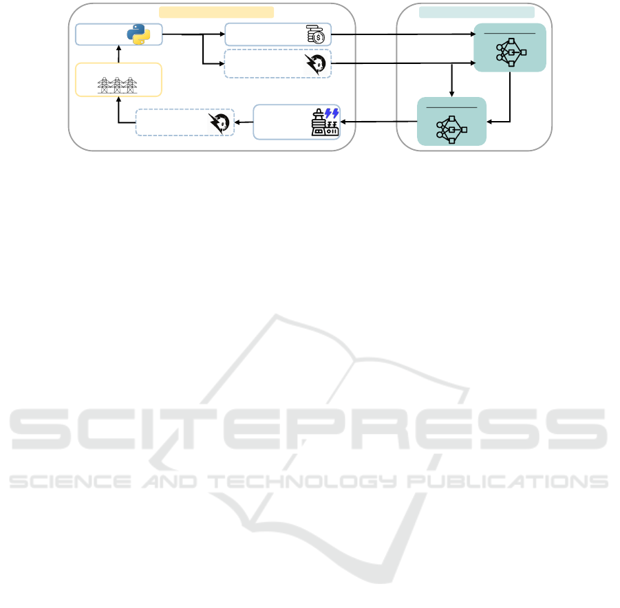
As illustrated in Figure 1, an agent is trained using

DRL. Over multiple timesteps, the agent iteratively

modiﬁes the generation values of a power grid, aim-

ing to maximize the reward. This reward reﬂects the

reduction in generation cost compared to the previous

timestep. The training process begins with a base case

where the agent minimizes the cost while optimizing

the search for feasible solutions. Once trained, this

agent can be deployed to compute OPF in power grids

with altered topologies, such as the loss of an electri-

cal line due to maintenance or the disconnection of a

load. The results obtained, in terms of cost, are often

better or comparable to those achieved using DCOPF.

4 BACKGROUND

In this section, we provide the necessary background

for GNN (subsection 4.1), the DRL algorithm used

(subsection 4.2) and we expand the deﬁnition of OPF.

Commonly, OPF minimizes the generation cost, so

the objective is to minimize the cost of power gen-

eration while satisfying operating constraints and de-

mands. Some of these constraints are restrictions of

both maximum and minimum voltage in the nodes or

that the net power in each bus is equal to the power

consumed minus generated (Mary et al., 2012). At the

same time, the Power Flow (PF) or load ﬂow refers to

the generation, load, and transmission network equa-

tions. It is a quantitative study to determine the ﬂow

of electric power in a network under given load condi-

tions whose objective is to determine the steady-state

operating values of an electrical network (Mary et al.,

2012).

4.1 Graph Neural Networks

Graph Neural Networks are methods based on deep

learning that function within the graph domain. Due

to their effectiveness, GNN has recently emerged as

a widely utilized approach for graph analysis (Zhou

et al., 2020a). The concept of GNN was ﬁrst intro-

duced by (Scarselli et al., 2009). This architecture can

be viewed as a generalization of convolutional neu-

ral networks tailored for graph structures, achieved

by unfolding a ﬁnite number of iterations. We em-

ploy Message Passing Neural Networks (MPNN), as

introduced in (Gilmer et al., 2017), which represents

a speciﬁc type of GNN that operates through an itera-

tive message-passing algorithm, facilitating the prop-

agation of information among elements in a graph

G = (N, E). Initially, the hidden states of the nodes

are set using the graph’s node-level features from the

data. Subsequently, the message-passing process un-

folds (Gilmer et al., 2017): Message (Equation 1),

Aggregation (Equation 1), and Update (Equation 2).

After a deﬁned number of message-passing steps, a

readout function r(·) takes the ﬁnal node states h

as input to generate the ultimate output of the GNN

model. The readout can predict various outcomes at

different levels, depending on the speciﬁc problem at

hand.

= a({m(h

, h

)}

i∈β(v)

) (1)

k+1

= u(h

, M

) (2)

4.2 Deep Reinforcement Learning

The objective in Reinforcement Learning (RL) is to

learn a behavior (policy). In RL, an agent acquires a

behavior through interaction with an environment to

achieve a speciﬁc goal (Schulman et al., 2017). This

approach is grounded in the reward assumption: all

objectives can be framed as the result of maximiz-

ing cumulative rewards. DRL is recognized for its ro-

bust ability to tackle complex decision-making chal-

lenges, making it suitable for capturing the dynamics

involved in the power ﬂow reallocation process (Li

et al., 2021).

Within the DRL algorithms, we use Proximal

Policy Optimization, formulated in 2017 (Schulman

et al., 2017) and becoming the default reinforcement

learning algorithm at OpenAI (Schulman et al., 2017)

because of its ease of use and its good performance.

As an actor-critic algorithm, the critic evaluates the

current policy and the result is used in the policy train-

ing. The actor implements the policy and it is trained

using Policy Gradient with estimations from the critic

(Schulman et al., 2017). PPO strikes a balance be-

tween ease of implementation, sample complexity,

and ease of tuning, trying to compute an update at

each step that minimizes the cost function while en-

suring that the deviation from the previous policy is

relatively small (Schulman et al., 2017). PPO uses

Trust Region and imposes policy ratio to stay within

a small interval (policy ratio r

is clipped), rt will

only grow to as much as 1 + ε (Equation 4) (Schul-

man et al., 2017). The total loss function for the PPO

comprises L

CLIP

(Equation 4), the mean-square error

Proximal Policy Optimization with Graph Neural Networks for Optimal Power Flow

349

Critic: GNN

Actor: GNN

Power grid case

AGENTENVIRONMENT

Compute cost

Reward

Action

𝑉

𝜋

(𝑠)

Compute

generation

Solve PF

Convert graph to

Pandapower net

Convert graph into

Pandapower net

State

Figure 1: Overview of the PPO-based architecture for power grid optimization. The system consists of an environment and

an agent. The environment simulates a power grid case. The agent, implemented using PPO with GNN, consists of an actor-

critic structure: the Actor-GNN selects actions, while the Critic-GNN evaluates state values. The agent interacts with the

environment by receiving state information, actions (change generation), and rewards based on the computed cost.

loss of the value estimator (critic loss), and an addi-

tional term that promotes higher entropy (enhancing

exploration) (Equation 3). PPO employs Generalized

Advantage Estimate (GAE) to compute the advantage

(

), as shown in Equation 5. This advantage method

is detailed in (Schulman et al., 2015).

TOTAL

= L

CLIP

+ L

VALUE

∗ k

− L

ENT ROPY

∗ k2 (3)

CLIP

(θ) =



min(r

(θ)

, clip(r

(θ), 1 − ε, 1 + ε)

)



(4)

GAE

= δ

+ (λγ)A

GAE

(5)

5 PROPOSED METHOD

In this section, we outline our approach, which is

schematically illustrated in Figure 1. Both the actor

and critic of the DRL agent are represented as GNN,

while the state of the environment corresponds to the

resulting graph of the power grid. Within the DRL en-

vironment, the agent executes an action at each time

step, adjusting the power of the generator. Subse-

quently, the power grid graph is updated through a

Power Flow.

We treat our power grid as graph-structured data

by utilizing information on the power grid topology,

where electrical lines serve as edges and buses as

nodes, along with the associated loads and genera-

tions. For the electrical lines, we deﬁne features using

resistance R and reactance X (e

ACLine

n,n

= [R

n,m

, X

n,m

]).

For the buses, we incorporate voltage information, in-

cluding its magnitude V and phase angle θ, as well

as the power exchanged at that bus between the con-

nected loads and generators, represented as X

, θ

, P

, Q

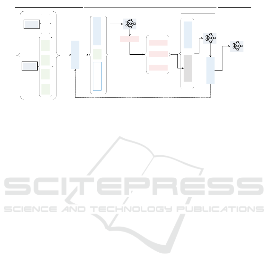
The overall architecture of the GNN is illustrated

in Figure 2, which includes the message passing and

readout components. At each message-passing step

k, each node v receives the current hidden states of

all nodes in its neighborhood and processes them in-

dividually by applying a message function m() (NN)

along with its own internal state h

and the features

of the connecting edge. These messages are then ag-

gregated through a concatenation of min, max, and

mean operations. By combining this message aggre-

gation with the node’s hidden state and updating the

combination using another NN, new hidden state rep-

resentations are generated. After a speciﬁed number

of message passing steps, a readout function r() takes

the ﬁnal node states h

as input to produce the ﬁnal

output of the GNN model.

For the actor, whose output is the RL policy, the

readout consists of a 3-layer MLP NN where the in-

put comprises each of the node representations. We

independently pass through this readout the represen-

tation of all nodes with a generator, resulting in N out-

put values. Each output value signiﬁes the probabil-

ity of selecting that generator to enhance its power.

This approach to managing the readout ensures that

the architecture remains generalizable to any num-

ber of generators. These values are utilized to form

a probability distribution, from which a value is sam-

pled (representing the ID of the generator whose gen-

eration is increased at that time horizon t). The critic

employs a centralized readout that takes all node hid-

den states as inputs (by concatenating the sum, min-

imum, and maximum), producing an output that es-

timates the value function. Consequently, the input

dimension is 3*node representation with a single out-

put for the entire graph. The critic is also structured

as a 3-layer MLP.

Regarding the environment with which the agent

interacts, at each time instant t, the state is deﬁned by

the graph updated by the Power Flow. In each horizon

step (t), the action performed by the agent involves in-

creasing the generation of one of the generator nodes.

The agent will determine which of the available gen-

DATA 2025 - 14th International Conference on Data Science, Technology and Applications

350

Step 1. Create embeddings

Eye-tracking

features

projector

Token-wise

conversion

1,1

1,2

1,n

2,1

2,2

1,n

t,1

t,2

t,n

…

RoBERTa

[CLS]

Step 2. Aggregate embeddings

Step 3. Compute reward

CONCAT

response 1

How do I make authentic

patatas bravas?

Input test

Best response

Frozen model

Embedding layer

…

[CLS]

Tok 1

…

Tok N

Linear

nFix

FFD

GPT TRT

fixProp

Preference

datasets

prompt

Worst response

…

response 2

response 3

response n

ADD

Remapping

Remapping between

tokenizers

Transformer decoder

only architecture

x N

Regression layer

[log(𝜎(𝑟

𝜃

𝑥, 𝑦

𝑤

− 𝑟

𝜃

(𝑥, 𝑦

𝑙

)))]

Passing aggregated

embedding as input to the

transformer decoder

Using the embedding

layer of the RM

Eye-tracking

datasets

Concatenating the

prompt with the best

and worst responses

to construct the

input test

Passing

concatenated

embedding as

input to the

transformer

decoder

Preference

datasets

Eye-tracking embedding

Text embedding

𝒇

𝟎

𝒇

𝟏

𝒇

𝒏

𝛉

min

max

sum

mean

Node

features

Edges

features

Prepare initial node representation

Message passing (k times)

Readout

𝒇

𝟎

𝒇

𝟏

𝒇

𝒏

𝒇

𝟎

𝒇

𝟏

𝒇

𝒏

message

min

max

message

mean

message

Create message

Aggregate messages

𝒇

𝟎

𝒇

𝟏

𝒇

𝒏

𝒇

𝟎

𝒇

𝟏

𝒇

𝒏

Update

Node representation

Neighbours' messages

Figure 2: GNN architecture. Both critic and actor employ the same GNN architecture, differing only in their readout layers.

The process initiates with the preparation of initial node representations, leveraging both node and edge features. Speciﬁcally,

the GNN’s input comprises the electrical parameters of the grid. During the message-passing phase (repeated k times), each

node generates messages based on its features, which are subsequently aggregated from its neighbors. These aggregated

messages reﬁne the node representations via an update function. Ultimately, in the readout phase, the actor utilizes these

reﬁned representations to compute the action, while the critic uses them to estimate the value function.

erators will have its generation increased by one por-

tion. For each generator, the power range between its

maximum and minimum power is divided into N por-

tions. When a generator reaches its maximum power,

generation cannot be increased, resulting in the power

grid (and thus the state of the environment) remaining

unchanged. If the PF does not converge, it indicates

that with the given demand and generation, meeting

the constraints is not feasible; we refer to this situ-

ation as an infeasible solution. When initializing an

episode (the initial state of the power grid), we aim

for the generation to be as low as possible, allowing

the agent to raise it until it reaches the optimum. Ad-

ditionally, we must consider that if the generation is

too low in the initial time steps, the solution may be-

come infeasible. Consequently, we decide to set the

minimum generation at 20%. The reward at time t is

calculated as the improvement in the solution’s cost

compared to t − 1, as shown in Equation 6. The re-

ward is positive during a time step when the agent’s

action results in a decrease in generation cost. Con-

versely, if the agent selects a generator that is already

at its maximum capacity, leads to an infeasible solu-

tion, or increases the cost, the reward will be negative.

r(t) =











MinMaxScaler(cost) − Last(MinMaxScaler(cost))

cte

if selected generator already in P

max

cte

if solution no feasible

(6)

6 PERFORMANCE EVALUATION

This section outlines the experimentation conducted

to validate the proposed approach, the data utilized,

and discusses the results obtained.

Overview: We train the agent using a base case

and subsequently evaluate its performance in modi-

ﬁed scenarios. On one hand, we adjust the number of

loads and their values, as real power grid operations

involve continuous changes in loads. On the other

hand, we simulate the unavailability of certain elec-

trical lines due to breakdowns or maintenance. This

approach demonstrates that the agent, once trained,

can generalize to previously unseen cases. We com-

pare the cost differences between our method and the

industry standard method, the DCOPF. Our goal is

to demonstrate that our method can produce a solu-

tion that is equal to or better than the DCOPF, while

avoiding its disadvantages.

6.1 Experimental Setting

We train the agent using the IEEE 30 bus system as

our case study (Figure 3). This system consists of

thirty nodes, forty links, ﬁve generators, and twenty

loads, with all generators modeled as thermal gener-

ators. We utilize Pandapower, a Python-based, BSD-

licensed power system analysis tool (Thurner et al.,

2018). This tool enables us to perform calculations

such as OPF using the IPOPT optimizer and PF analy-

sis, which we employ to evaluate our costs and update

our environment. Additionally, this library allows us

Proximal Policy Optimization with Graph Neural Networks for Optimal Power Flow

351

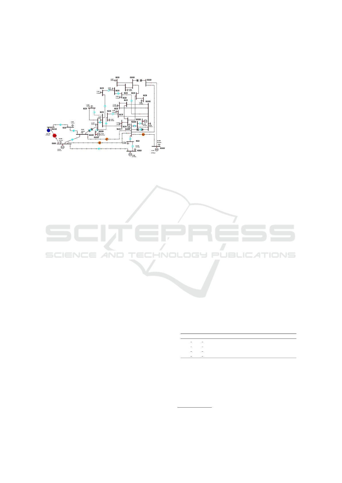
to verify the physical feasibility of our solutions by

ensuring they comply with PF constraints.

Figure 3: IEEE 30 bus system (Fraunhofer, 2022).

The objective of the training is to optimize the pa-

rameters so that the actor becomes a good estimator of

the optimal global policy and the critic learns to ap-

proximate the state value function of any global state.

Many hyperparameters can be modiﬁed, and they are

divided into different groups. Grid search has been

performed on many of them, and the ﬁnal selected

values of the most important ones are shown below.

• Related to learning loop: Minibatch (25), epochs

(3) and optimizer (ADAM), with its parameters

like learning rate lr (0.003).

• Related to the power grid: Generator portions

(50).

• Related to RL: Episodes (500), horizon size T

(125), reward cte

(-1) and cte

(-2).

• Actor and Critic GNN: Message iterations k (4),

node representation size (16). The NN to create

the messages is a 2-layer MLP and the updated

one is 3-layer MLP.

PPO is an online algorithm that, similar to other re-

inforcement learning algorithms, learns from experi-

ence. The training pipeline is organized as follows:

• An episode of length T is generated by fol-

lowing the current policy. While at the same

time the critic’s value function V evaluates each

visited global state; this deﬁnes a trajectory

{

, a

, r

, p

, V

, s

t+1

}

T −1

t=0

• This trajectory is used to update the model pa-

rameters –through several epochs of minibatch

Stochastic Gradient Descent– by maximizing the

global PPO objective.

The same process of generating episodes and updat-

ing the model is repeated for a ﬁxed number of iter-

ations to guarantee convergence. MinMaxScaler has

been used for data preprocessing for node features,

edge features and generation output. More implemen-

tation details can be found in the public repository

6.2 Experimental Results

Once the training has been done and the best com-

bination of hyperparameters, network design and re-

ward modelling has been chosen, the best checkpoint

of the model is selected to compute OPF in different

networks. To validate our solution, we use the devi-

ation of the cost concerning the minimum cost, the

one obtained with the ACOPF (%DRL+OPF perf. in

Table 1 - Table 3). We compare it with the cost devia-

tion obtained with DCOPF (%DCOPF perf in Table 1

- Table 3). We compute the ratio between these two

deviations. We calculate the improvement ratio by di-

viding the ﬁrst value by the second, which reﬂects the

enhancement over the DCOPF.

Once the model is trained, only the actor part is

used in the evaluation. During T steps of an episode,

the actions sampled from the probability distribution

obtained from the actor for each state of the network

are executed. Finally, the mean cost of the best ten

evaluations is measured, as well as the convergence of

the problem. We evaluate 100 times for each test case.

In Table 1 - Table 3, it is highlighted between the devi-

ation in % of our solution concerning the OPF’s one

and the deviation obtained by the DCOPF. We also

assess the convergence and physical feasibility of our

solution, ﬁnding that it was feasible in the majority of

cases.

First, all network loads are varied by multiplying

their value by a random number between a value less

than 1 and a value higher than 1 (Table 1). Each row in

the table is a test in which the name speciﬁes the up-

per and lower percentages by which loads have been

varied. In all tests, performance with our method is

better with ratios of up to 1.30.

Table 1: Results on case IEEE 30 varying loads from base

case.

% DRL+OPF perf. %DCOPF perf. ratio

load inf0.1 sup0.1 0,75 0,77 1,02

load inf0.2 sup0.1 0,59 0,68 1,16

load inf0.3 sup0.1 0,53 0,73 1,38

load inf0.4 sup0.1 0,61 0,67 1,10

After varying the load value, we experiment with

removing n loads from the grid. We randomly choose

several loads, remove them from the network and

evaluate the model (Table 2). Each row in the ta-

ble is a test in which the name speciﬁes the number

of loads that have been removed. Our cost deviation

https://github.com/anlopez94/opf_gnn_ppo

DATA 2025 - 14th International Conference on Data Science, Technology and Applications

352

is lower or similar than the DCOPF even by elimi-

nating almost 50% of the loads. Finally, in Table 3

we show the results of creating networks from the

original one by removing one or more electrical lines

(edges). Each row in the table is a test in which the

name speciﬁes the number of power lines removed.

Table 2: Results on case IEEE 30 removing loads from base

case.

% DRL+OPF perf. %DCOPF perf. ratio

load 1 0,67 0,72 1,07

load 2 0,71 0,71 1,00

load 3 0,67 0,67 1,00

load 4 1,06 0,68 0,65

load 5 0,61 0,64 1,05

load 8 1,10 0,63 0,52

Table 3: Results on case IEEE 30 removing edges from base

case.

% DRL+OPF perf. %DCOPF perf. ratio

edge 1 0,73 0,77 1,05

edge 2 0,41 1,16 2,83

edge 3 0,62 0,61 0,99

edge 4 0,65 0,88 1,36

edge 5 0,90 0,96 1,07

edge 8 0,59 0,89 1,51

In experiments removing electrical lines (Table 3)

as more power lines are removed (more than 8), some-

times, the agent does not ﬁnd a good feasible solu-

tion (no convergence). When we experimented with

changing the load values in the second test (Table 1),

we observed that increasing the loads by more than

10% caused the tests to fail to converge. With the

other changes in topology, 100% of tests converged,

so we can conclude that our model is capable of gen-

eralizing to unseen topologies (based on the trained

one).

7 DISCUSSION

We have successfully designed a solution to address

the OPF, capable of generalization, utilizing DRL and

GNN. The network topology has been modiﬁed, and

we have demonstrated that the agent can identify a

strong solution (with performance closely aligned to

the current industry standard DCOPF), ensuring that

this solution is both feasible and compliant with the

constraints. Thanks to the design of GNN, it can be

trained on various cases and subsequently applied to

different scenarios. In this paper, we validate that this

architecture effectively tackles OPF, showcasing the

generalization capability of our solution by consid-

ering modiﬁcations to the network scenario encoun-

tered during training (including different loads and

a reduction in the number of edges). By integrating

these two technologies for the ﬁrst time, we conclude

that their combination is feasible, leveraging the ad-

vantages of both. Our ﬁndings indicate that the pro-

posed architecture represents a promising initial step

toward solving the OPF. Future work could explore

the incorporation of additional features in the node

representation, such as the maximum and minimum

allowable voltage and model other types of electrical

generation.

ACKNOWLEDGMENTS

This research is supported by the Industrial Doctorate

Plan of the Department of Research and Universities

of the Generalitat de Catalunya, under Grant AGAUR

2023 DI060.

REFERENCES

Cao, D., Hu, W., Xu, X., Wu, Q., Huang, Q., Chen, Z.,

and Blaabjerg, F. (2021). Deep reinforcement learning

based approach for optimal power ﬂow of distribution

networks embedded with renewable energy and stor-

age devices. Journal of Modern Power Systems and

Clean Energy, 9(5):1101–1110.

Diehl, F. (2019). Warm-starting ac optimal power ﬂow with

graph neural networks. In 33rd Conference on Neu-

ral Information Processing Systems (NeurIPS 2019),

pages 1–6.

Donnot, B., Guyon, I. M., Schoenauer, M., Marot, A., and

Panciatici, P. (2017). Fast power system security anal-

ysis with guided dropout. ArXiv, abs/1801.09870.

Donon, B., Cl

ement, R., Donnot, B., Marot, A., Guyon,

I., and Schoenauer, M. (2020). Neural networks for

power ﬂow: Graph neural solver. In Electric Power

Systems Research, volume 189, page 106547.

Donon, B., Donnot, B., Guyon, I., and Marot, A. (2019).

Graph Neural Solver for Power Systems. In IJCNN

2019 - International Joint Conference on Neural Net-

works, Budapest, Hungary.

Fraunhofer, IEE, U. o. K. (2022). Pandapower documenta-

tion.

Gilmer, J., Schoenholz, S. S., Riley, P. F., Vinyals, O., and

Dahl, G. E. (2017). Neural message passing for quan-

tum chemistry. In International conference on ma-

chine learning, pages 1263–1272. PMLR.

Li, J., Zhang, R., Wang, H., Liu, Z., Lai, H., and Zhang,

Y. (2021). Deep reinforcement learning for optimal

power ﬂow with renewables using graph information.

ArXiv, abs/2112.11461.

Liao, W., Bak-Jensen, B., Pillai, J. R., Wang, Y., and Wang,

Y. (2022). A review of graph neural networks and

Proximal Policy Optimization with Graph Neural Networks for Optimal Power Flow

353

their applications in power systems. Journal of Mod-

ern Power Systems and Clean Energy, 10(2):345–360.

Mary, A., Cain, B., and O’Neill, R. (2012). History of opti-

mal power ﬂow and formulations. Fed. Energy Regul.

Comm., 1:1–36.

Munikoti, S., Agarwal, D., Das, L., Halappanavar, M., and

Natarajan, B. (2024). Challenges and opportunities

in deep reinforcement learning with graph neural net-

works: A comprehensive review of algorithms and ap-

plications. IEEE Transactions on Neural Networks

and Learning Systems, 35(11):15051–15071.

Owerko, D., Gama, F., and Ribeiro, A. (2020). Optimal

power ﬂow using graph neural networks. In ICASSP

2020 - 2020 IEEE International Conference on Acous-

tics, Speech and Signal Processing (ICASSP), pages

5930–5934.

Pan, X., Chen, M., Zhao, T., and Low, S. H. (2022). Deep-

opf: A feasibility-optimized deep neural network ap-

proach for ac optimal power ﬂow problems. In IEEE

Systems Journal, pages 1–11.

Scarselli, F., Gori, M., Tsoi, A. C., Hagenbuchner, M.,

and Monfardini, G. (2009). The graph neural net-

work model. IEEE Transactions on Neural Networks,

20:61–80.

Schulman, J., Moritz, P., Levine, S., Jordan, M., and

Abbeel, P. (2015). High-dimensional continuous con-

trol using generalized advantage estimation. ArXiv,

abs/1506.02438.

Schulman, J., Wolski, F., Dhariwal, P., Radford, A., and

Klimov, O. (2017). Proximal policy optimization al-

gorithms. ArXiv, abs/1707.06347.

Thurner, L., Scheidler, A., Sch

afer, F., Menke, J.-H., Dol-

lichon, J., Meier, F., Meinecke, S., and Braun, M.

(2018). Pandapower—an open-source python tool for

convenient modeling, analysis, and optimization of

electric power systems. IEEE Transactions on Power

Systems, 33(6):6510–6521.

Wood, A. J., Wollenberg, B. F., and Sheble, G. B. (2013).

Power Generation, Operation, and Control. John Wi-

ley & Sons, Hoboken, NJ, USA, 3rd edition.

Zhen, H., Zhai, H., Ma, W., Zhao, L., Weng, Y., Xu,

Y., Shi, J., and He, X. (2022). Design and tests of

reinforcement-learning-based optimal power ﬂow so-

lution generator. Energy Reports, 8:43–50. 2021 The

8th International Conference on Power and Energy

Systems Engineering.

Zhou, J., Cui, G., Hu, S., Zhang, Z., Yang, C., Liu, Z.,

Wang, L., Li, C., and Sun, M. (2020a). Graph neu-

ral networks: A review of methods and applications.

AI Open, 1:57–81.

Zhou, Y., Zhang, B., Xu, C., Lan, T., Diao, R., Shi, D.,

Wang, Z., and Lee, W.-J. (2020b). A data-driven

method for fast ac optimal power ﬂow solutions via

deep reinforcement learning. Journal of Modern

Power Systems and Clean Energy, 8(6):1128–1139.

DATA 2025 - 14th International Conference on Data Science, Technology and Applications

354