CCR-Logistic Based Variable Importance Visualization: Differentiating

Prime and Suppressor Variables in Logit Models

Ana Peri

1,2 a

and Ivan Sever

3 b

Faculty of Science, University of Split, Split, Croatia

Sibenik University of Applied Sciences, Sibenik, Croatia

Institute for Tourism, Zagreb, Croatia

Keywords:

Variable Importance Visualisation, Logistic Regression, Correlated Component Regression, Suppression.

Abstract:

Logistic regression typically involves assessing variable importance. This task becomes considerably more

challenging in the presence of correlated variables (predictors) and suppression. We present a procedure for

determining variable importance in multiple logistic regression models that can distinguish between suppres-

sor variables and prime predictors. We propose a simple visualization tool for representing variable importance

that can help practitioners to determine important prime and suppressor variables when building the multiple

logistic regression model. The methodology relies on the extension of the Correlated Component Regression

approach to logistic regression (CCR-Logit), which utilizes linear combinations of predictors instead of orig-

inal predictors and can easily be generalized to various regression models. CCR-logistic methodology can

handle a large number of predictors and is especially useful when dealing with correlated predictors. The vari-

able importance is quantiﬁed by observing standardized regression coefﬁcients from univariate models and

higher-order component models, where univariate models capture the direct effect on the outcome, while the

higher-order component models capture the suppressor effects. The proposed methodology is presented on a

real-world dataset within the ﬁeld of tourism.

1 INTRODUCTION

When building a regression model it can be more ef-

ﬁcient to select a subset of relevant predictors, than to

build a regression model on a large set of all possi-

ble variables. There are several reasons for this, from

the theoretical and practical side. From the practi-

cal side, simple models are more effective than com-

plex models, more cost-efﬁcient and time-efﬁcient,

are easier to interpret, and often are more stable on

out-of-sample data. On the theory side, good theories

are parsimonious, containing only those constructs

essential for understanding a certain phenomenon of

interest (Braun and Oswald, 2011). Thus, assess-

ing variable importance is essential when building re-

gression models. A detailed review of various vari-

able importance metrics developed for linear models

together with several important properties that vari-

able importance metrics should satisfy can be found

in Gr

omping (2015).

https://orcid.org/0000-0001-9180-0270

https://orcid.org/0000-0002-7043-4862

Various metrics and approaches for variable im-

portance assessment in logistic regression have been

developed. The most widely adopted approaches in-

clude standardized regression coefﬁcients which of-

ten rely on different approaches to standardization

(see for instance Menard (2004)). Also, a popular

method for evaluating predictor importance is dom-

inance analysis where one predictor is considered as

more important than another if it contributes more to

the prediction of the criterion than does its competitor

at a given level of analysis (Azen and Traxel, 2009).

Moreover, the analyses often include calculating test

values, information, and prediction performance mea-

sures for nested models (such as performing the LR

test or comparing AIC, BIC, AUC for a model that

includes and model that does not include a variable

of interest). Some model-building strategies can be

found in Hosmer and Lemeshow (2000). As in the

general case, when building prediction models and as-

sessing feature importance, there is no deﬁnitive or

unambiguous method for establishing predictor im-

portance (Braun and Oswald, 2011).

Assessing variable importance in logistic regres-

Periši

c, A., Sever and I.

CCR-Logistic Based Variable Importance Visualization: Differentiating Prime and Suppressor Variables in Logit Models.

DOI: 10.5220/0013461700003967

In Proceedings of the 14th International Conference on Data Science, Technology and Applications (DATA 2025), pages 43-52

ISBN: 978-989-758-758-0; ISSN: 2184-285X

sion with a large set of potential predictors is not

straightforward. Similar to multiple linear regression,

the relative importance of a predictor variable in lo-

gistic regression can vary depending on the subset of

predictor variables included in the model (Azen and

Traxel, 2009). Moreover, assessing predictor impor-

tance becomes more challenging in the presence of

suppression. A suppressor variable shares no vari-

ance directly with the dependent variable and thus

contributes to the regression model through remov-

ing irrelevant variance from the other independent

variables (Nathans et al., 2012). There are differ-

ent approaches to deﬁning a suppressor variable, and

thus different approaches for identifying a suppres-

sor variable in the regression model (see for instance

Friedman and Wall (2005); Ludlow and Klein (2014);

Shieh (2006); Velicer (1978)). Some of the common

approaches include observing regression coefﬁcients

and corresponding t-statistics. For instance, some ap-

proaches suggest that suppression exists if the squared

multiple regression coefﬁcient for a particular predic-

tor is higher than the squared univariate regression co-

efﬁcient for the same predictor. Instead of multiple

regression coefﬁcient and squared univariate regres-

sion coefﬁcient, we can also evaluate the t-statistics of

the estimated coefﬁcient. Also, some approaches sug-

gested observing the changes in the estimated regres-

sion coefﬁcients when adding new predictors: sup-

pression is present if the change in the estimated re-

gression coefﬁcient of a predictor is signiﬁcant when

adding a new predictor into the model. Other ap-

proaches suggest that variable X

is a suppressor when

the squared multiple correlation coefﬁcient of Y with

all predictors X

, X

, . . . , X

is larger than the sum of

the squared multiple correlation coefﬁcient of Y with

all predictors except X

, and the squared correlation

coefﬁcient of Y and X

A powerful tool in understanding regression

models is visualization. Variable importance in

regression models is mostly visualized through

bar plots and line plots that present the variable

importance metric. Visualizations that exceed the

one-dimensional aspect of presenting variable impor-

tance have also been developed. For instance, Inglis

et al. (2022) constructed heatmap and graph-based

displays showing variable importance and interaction

jointly.

In this work, we present a visualization tool that

presents variable importance in a logistic regression

model and distinguishes between the direct and indi-

rect variable effects. The proposed methodology is

capable of handling a large set of correlated predic-

tors. Along with distinguishing between the direct

and indirect effects, the proposed visualization covers

three dimensions of interest when evaluating a predic-

tor: statistical signiﬁcance, its total effect and direc-

tion of the relationship. We introduce the methodol-

ogy in the second section and present the application

to a real-world problem in section 3.

2 PROPOSED METHODOLOGY

The methodology for visualizing variable importance

presented in this work relies on the Correlated Com-

ponent Regression (CCR) method. The CCR method,

introduced by Magidson J. (Magidson, 2010, 2013), is

a dimension reduction method developed for multiple

regression models that utilizes K < P correlated lin-

ear combinations of the predictors instead of the orig-

inal P predictors, to predict an outcome variable. The

ﬁrst component captures the effects of predictors that

have a direct effect on the outcome, while the higher-

order components capture indirect effects, i.e. the ef-

fects of suppressor variables that improve prediction

by removing extraneous variation from one or more of

the predictors that have direct effects. This approach

identiﬁes prime predictors as those having substantial

loadings on the ﬁrst component, and suppressor vari-

ables as those having substantial loadings on higher-

order components, and relatively small loadings on

the ﬁrst component (Magidson, 2013). For instance,

in the case of two components, pure suppressor vari-

ables have zero loadings on the ﬁrst but highly signiﬁ-

cant loadings on the second CCR component (Magid-

son, 2010).

The CCR algorithm is developed for multiple re-

gression models and has different variants depending

on the scale type of the outcome variable. For in-

stance, when the outcome variable is dichotomous,

we can apply the CCR-logistic regression (CCR-

Logit) approach. The easiest way of adapting the

CCR methodology to the logistic regression case is

performing the logit transformation of the outcome

variable and then evaluating the model as the mul-

tiple linear regression model. We ﬁrst present the

CCR algorithm extended to logistic regression (CCR-

Logistic) introduced in Magidson (2013). Also, we

present the approach for identifying prime and sup-

pressor variables.

Assume we have a collection of X

, X

, . . . , X

predictor variables and we are building a logistic re-

gression model where the dichotomous outcome vari-

able is denoted by Y . For ease of understanding, we

denote the logit transformation Logit(Y ) simply by

Y . The algorithm is executed through the following

steps, denoted as S

to S

DATA 2025 - 14th International Conference on Data Science, Technology and Applications

S1. Univariate Models

Step 1.1. Estimate P univariate models

For each predictor X

, i = 1, 2, . . . , P, estimate the

univariate model

Y = β

+ λ

(1)

+ ε

Here, β

represents the intercept, ε

is the er-

ror term, λ

(1)

is the univariate regression coef-

ﬁcient of interest that captures the direct effect

of the predictor variable X

on the outcome. For

each predictor X

, i = 1, 2, . . . , P, check the asso-

ciated p-value and denote it by pv

(1)

. The associ-

ated p-values are measures of signiﬁcant direct ef-

fects. Predictors that have signiﬁcant coefﬁcients

are considered as prime predictors (here we take

(1)

< 0.1, but this bound can be changed).

Step 1.2. Univariate regression coefﬁcient stan-

dardization

For each predictor X

, i = 1, 2, . . . , P, standardize

the univariate regression coefﬁcients by calculat-

ing:

∗(1)

= λ

(1)

, i = 1, 2, . . . , P

where λ

(1)

is the regression coefﬁcient estimated

in the univariate regression model, and σ

is the

standard deviation of the predictor X

S2. Higher Order Components

Step 2.1. Estimate the ﬁrst component

The ﬁrst component S

is deﬁned as the weighted

linear combination of P predictors, with weights

being proportional to estimated coefﬁcients λ

(1)

∑

i=1

(1)

The ﬁrst component captures the total direct effect

of all predictors.

Step 2.2. Estimate the higher-order components

For k = 2, . . . , K < P, deﬁne the k-th component S

as the weighted average of all 1-predictor partial

effects:

∑

i=1

(k)

where weights λ

(k)

are estimated from the regres-

sion models:

Y = α

+ γ

(k)

1.i

+ ··· + γ

(k)

(k−1).i

k−1

+ λ

(k)

+ ε

i = 1, 2, . . . , P. Higher-order components cap-

ture the effect of suppressor variables that im-

prove predictions by removing extraneous varia-

tion from prime predictors. For each λ

(k)

, i =

1, 2, . . . , P, check the associated p-value and de-

note it by pv

(k)

. The associated p-values are mea-

sures of signiﬁcant suppressor effect. Predictors

that have at least one signiﬁcant coefﬁcient λ

(k)

for k = 2, . . . , K (pv

(k)

< 0.1) are considered sup-

pressor predictors.

Step 2.3. The standardized coefﬁcient

For each predictor X

, i = 1, 2, . . . , P, calculate the

standardized coefﬁcient

∗(k)

= λ

(k)

, i = 1, 2, . . . , P, k = 2, . . . , K.

S3. The ﬁnal K-component model

Step 3.1. The Final K-Component Model

Estimate the ﬁnal K-component model, which is

deﬁned as a regression model with outcome Y and

predictors S

, S

, . . . , S

Y = α

(K)

∑

k=1

(K)

+ ε

Step 3.2. Regression coefﬁcients for the predic-

tors

The predicted values of the outcome variables are

then:

Y = α

(K)

∑

k=1

(K)

and can then be easily re-expressed to obtain re-

gression coefﬁcients for the predictors by substi-

tuting as follows:

Y = α

(K)

∑

k=1

(K)

∑

i=1

(k)

= α

(K)

∑

i=1

The coefﬁcient β

for predictor X

is the weighted

sum of the loadings, where the weights are the re-

gression coefﬁcients of the components in the K-

component model:

∑

k=1

(K)

(k)

Step 3.3. Standardized ﬁnal CCR coefﬁcients

Calculate the associated standardized coefﬁcient

as:

∗

= β

, i = 1, 2, . . . , P.

The optimal number of components and predictors

involved can be found by performing cross-validation

on the training dataset. Results from simulations and

applications with real high-dimensional data suggest

that CCR models rarely require more than 10 compo-

nents regardless of the number of predictors and usu-

ally perform well with 3 or 4 components, while the

estimation is fast (Magidson (2010)).

Having the results of the CCR-Logit algorithm,

we establish the visualization in the Cartesian coor-

dinate system by covering 5 dimensions of interest:

CCR-Logistic Based Variable Importance Visualization: Differentiating Prime and Suppressor Variables in Logit Models

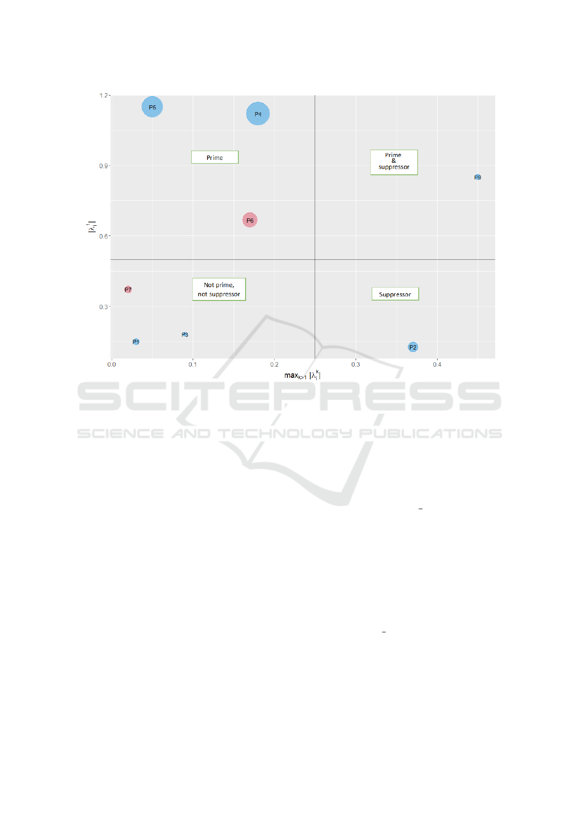
Figure 1: Proposed visualization.

(D1) (Prime/Direct Effect)

We observe the direct impact of each variable on

the outcome by presenting the absolute value of

the standardized univariate regression coefﬁcient

∗(1)

on the y-axis. Variables that have signiﬁ-

cant univariate regression coefﬁcients are consid-

ered as signiﬁcant prime predictors.

(D2) (Suppressor Effect)

We observe the indirect impact of each variable

on the outcome by presenting the largest abso-

lute value of the standardized regression coefﬁ-

cient λ

∗(k)

, k > 1 on the x-axis, i.e. we present

∗(Amax)

= max

k>1

|λ

∗(k)

|. Variables that have at least

one signiﬁcant λ

∗(k)

coefﬁcient are considered as

signiﬁcant suppressor predictors.

(D3) (Statistical Signiﬁcance)

In the proposed visualization, each variable is pre-

sented by a data point (λ

∗(Amax)

, |λ

∗(1)

|). The sig-

niﬁcance of each variable is captured by associ-

ated p-values (min

k>1

(k)

, pv

(1)

). Following this

simple visualization strategy, we consider a cat-

egorization of a variable into 4 cases: a pre-

dictor can be a (I) a signiﬁcant prime predic-

tor, (II) a signiﬁcant suppressor predictor, (III)

both a signiﬁcant prime and a signiﬁcant sup-

pressor predictor, and (IV) a nonsigniﬁcant prime

and a nonsigniﬁcant suppressor. Thus, we divide

the visualization area into four quadrants accord-

ing to the signiﬁcance of the predictors in the

univariate and higher-order models. The verti-

cal line is placed at x =

(λ

+ λ

) where λ

is the highest value of the standardized coefﬁ-

cients λ

∗(Amax)

for the variables that had no sig-

niﬁcant coefﬁcients in the higher-order compo-

nents, i.e. we take λ

= max

not suppressor

∗(Amax)

while λ

is the lowest value of standardized coef-

ﬁcients λ

∗(Amax)

for the predictors that had signif-

icant coefﬁcients in the higher-order components,

i.e. λ

= min

suppressor

∗(Amax)

. The horizontal line

is placed at y =

(λ

+ λ

), where λ

is the

lowest absolute value of the univariate standard-

ized coefﬁcient |λ

∗(1)

| of the univariate signiﬁcant

predictors, i.e. λ

= min

prime

|λ

∗(1)

|, while λ

the highest absolute value of the univariate stan-

dardized coefﬁcients |λ

∗(1)

| of the univariate non-

DATA 2025 - 14th International Conference on Data Science, Technology and Applications

signiﬁcant predictors, i.e. λ

= max

not prime

|λ

∗(1)

(D4) (Overall Effect)

The overall effect of each predictor on the out-

come is visualized by the size of each data point

associated with the predictor. The size of each

data point is proportional to the normalized value

of the associated absolute value of the ﬁnal stan-

dardized coefﬁcient β

∗

from the ﬁnal CCR model.

The normalized value is calculated as

NORMβ

∗

∑

i=1

|β

∗

|β

∗

(D5) (Direction)

The visualization is enriched by adding the in-

formation on the direction of the (overall) rela-

tionship between the predictor and the outcome

variable. This is achieved by presenting positive

ﬁnal standardized coefﬁcients in one color, and

negative ﬁnal standardized coefﬁcients in another

color.

The example of such a visualization is presented

in Figure 1. The Figure is divided into four areas

distinguishing between the (signiﬁcant) pure prime,

(signiﬁcant) pure suppressor, (signiﬁcant) prime and

suppressor, and nonsigniﬁcant variables. Predictors

having a positive overall effect on the outcome are

presented in blue, while predictors having a negative

overall effect are presented in red. The size of each

dot is proportional to the absolute value of the overall

effect. In this theoretical example, we have a collec-

tion of 8 variables included in the regression analysis.

Three variables, P5, P4 and P6 have a signiﬁcant di-

rect effect on the outcome. Predictors P4 and P5 have

the largest overall effect on the outcome and are pos-

itively related to the outcome. Predictor P6 is nega-

tively related to the outcome. Predictor P2 is a (pure)

suppressor variable, positively related with the out-

come. Predictor P8 has both direct and indirect effect

on the outcome. The overall effect of the predictor P8

on the outcome is positive. This hypothetical example

classiﬁes three variables as both nonsigniﬁcant prime

and nonsigniﬁcant suppressor variables, meaning that

these variables should be excluded from the regres-

sion analysis. Note that this example is theoretical

and that in practice we expect that the number of both

not prime and not suppressor variables should be low.

In fact, when dealing with carefully planned analyses

(this means that the variables (predictor candidates)

included in the regression analysis are carefully se-

lected) we expect that the selected variables will have

direct, indirect or both direct and indirect effect on the

outcome.

3 APPLICATION

We present the application of the proposed method-

ology on a real-world dataset from the survey on res-

idents’ perceptions of tourism impacts and their at-

titudes toward tourism in the city of Split, Croatia.

Split is the second-largest city in Croatia and the

largest Croatian city on the Adriatic coast, with ap-

proximately 160,000 inhabitants. As a Mediterranean

city with exceptional cultural-historical heritage and

natural beauty, Split is a highly attractive tourist des-

tination. In 2022, 2.6 million overnight stays were

realized in its commercial accommodation facilities.

The intensive growth of tourism over the past decade

has put a lot of pressure on residents’ well-being and

their living environment (Mate

c et al., 2022). The

survey of local residents in the city of Split, which

was conducted in June 2022 on a sample of 385 re-

spondents, was designed to identify the key drivers

of adverse tourism impacts in the city and thus sup-

port effective monitoring, management, and mitiga-

tion of risks associated with overtourism. The sample

was representative at the city level by gender and age

group of residents. Computer Assisted Telephone In-

terview (CATI) was used as a data collection method.

The dataset comprises eleven variables related to

residents’ perceptions of tourism impacts in the city

of Split. A detailed description of included variables

(i.e., impact indicators) can be found in the Appendix.

Six numerical variables are used in their original form

where Appearance, Apartmentization, Authenticity,

Space, and Services are responses to a 5-point rat-

ing scale, while Displacement is a binary variable.

Other four numerical variables F1:Social crowding,

F2:Waste and cleanliness, F3:Current expenses, and

F4: Housing affordability are constructed through ex-

ploratory factor analysis. Factors F1:Social crowding

and F2:Waste and cleanliness were established by per-

forming factor analysis on the set of crowding-related

variables: Noise, Trafﬁc, Crowding, Transport, Lit-

tering, Smell, Tourist behavior and Parking. Factors

F3:Current expenses and F4: Housing affordability

are constructed through exploratory factor analysis

applied on a set of price-related tourism impact items:

Housing affordability, Realestate prices, Rent, Utility

prices, Grocery prices, and Restaurant prices. These

ten variables are (theoretically) assumed to affect the

outcome variable. The outcome variable Perception is

a binary variable that presents the perception of over-

all tourism impacts. It is formed by categorizing the

overall attitude toward tourism impacts, measured on

a 5-point Likert scale anchored by very negative and

very positive, as either positive or neutral/negative.

CCR-Logistic Based Variable Importance Visualization: Differentiating Prime and Suppressor Variables in Logit Models

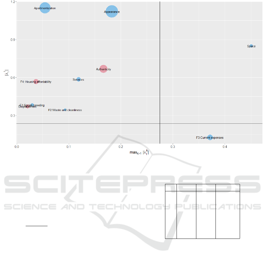
Figure 2: CCR-logit visualization example: tourism data.

The goal of the analysis is to build a model that ex-

plains the perception of overall tourism impacts by

using the set of ten aforementioned variables. Since

the outcome variable is a binary variable, it is reason-

able to conduct logistic regression analysis, where we

estimate the model

log



P(Y = 1)

P(Y = 0)



= β

+ β

+ . . . + β

that best explains the outcome. This also means se-

lecting the most important predictors and explaining

the relationship of each predictor with the outcome.

For this reason, we perform the CCR-Logit based vi-

sualization.

Before applying the CCR-Logit algorithm we de-

termined the value for the number of components

K that provides the optimal amount of regulariza-

tion. We chose the CCR model that maximizes the

cross-validated area under the curve (AUC), accuracy

(ACC) and sensitivity (SENSI).

We performed the cross-validation by splitting the

data into 10 exclusive partitions. Each partition was

used for test-training split where we estimate the

model with K components (K = 1, 2, . . . , 7). For each

number of components K, K = 1, 2, . . . , 7 we aver-

aged the performance metrics as presented in Table 1.

Based on 10-predictor models, the model with K = 2

components provides the maximum mean prediction

metrics values.

Table 1: Performance metrics for different values of K.

K AUC ACC SENSI

1 0.86 0.73 0.76

2 0.86 0.76 0.80

3 0.86 0.75 0.79

4 0.86 0.76 0.79

5 0.86 0.76 0.79

6 0.86 0.76 0.79

7 0.86 0.76 0.79

We estimated the two-component CCR model.

The estimated coefﬁcients λ

(k)

, standardized coefﬁ-

cients λ

∗(k)

, and the associated p-values pv

(k)

, for

k = 1, 2 and i = 1, . . . , 10, are presented in Table 2.

Also, we present the standardized value of the ﬁnal

coefﬁcient β

∗

in the same table.

The visualization of the results prepared accord-

ingly to the proposed methodology in the second sec-

tion is presented in Figure 2. Several conclusions

can be drawn from this visualization. Three main

prime predictors are Apartmentization, Appearance,

and Authenticity. These predictors are located in the

Prime area and have the largest overall effect. Pre-

dictors Apartmentization and Appearance have a pos-

itive overall effect on Perception, while Authenticity

has a negative overall effect due to coding. Predictors

F4:Housing affordability, Services, F1:Social crowd-

ing, F2:Waste and cleanliness, and Displacement are

DATA 2025 - 14th International Conference on Data Science, Technology and Applications

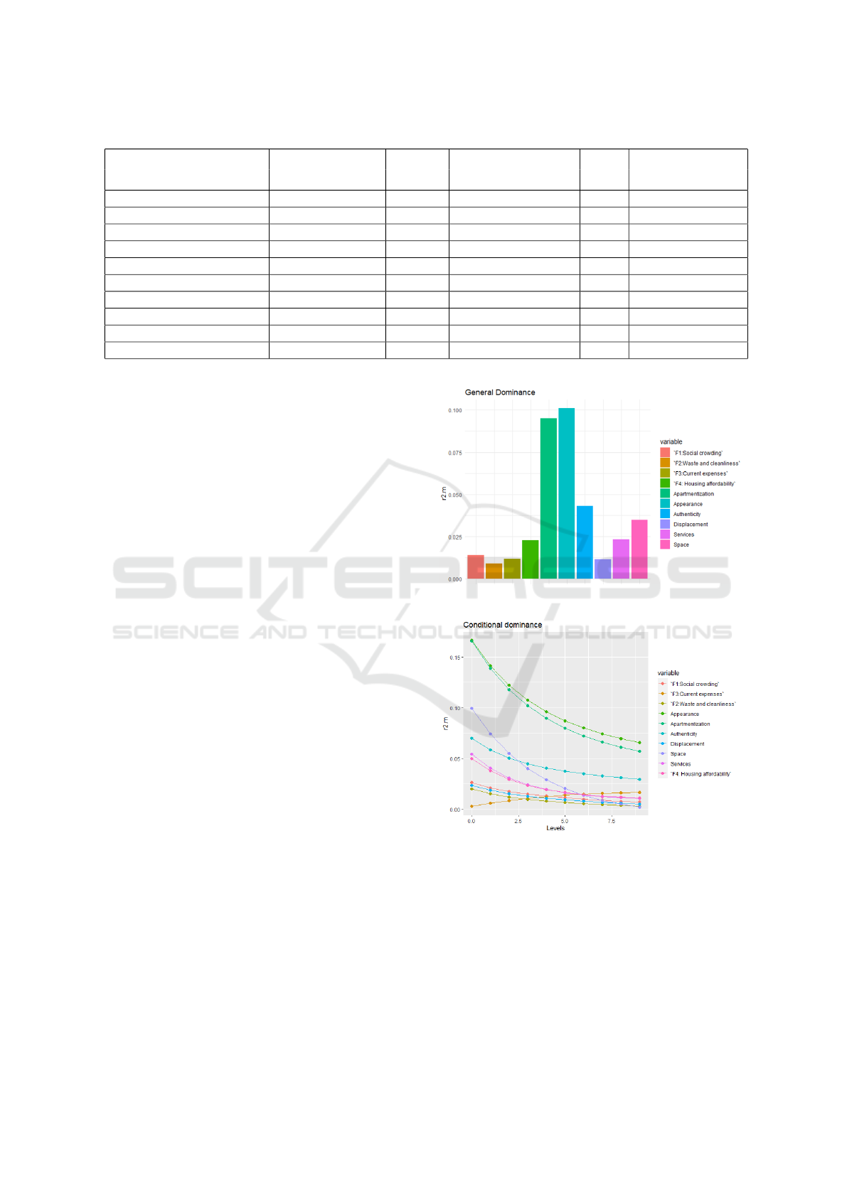
Table 2: Estimated coefﬁcients, p-values, and ﬁnal coefﬁcients for the two-component CCR model.

Predictor First component pv

(1)

Second component pv

(2)

Final coefﬁcients

∗(1)

∗(2)

∗

Apartmentization 1.149 < 0.001 0.05 0.809 0.853

Appearance 1.121 < 0.001 0.18 0.383 0.94

Authenticity -0.667 < 0.001 -0.17 0.338 -0.607

Space 0.850 < 0.001 -0.45 0.053 0.226

Services 0.585 < 0.001 -0.12 0.509 0.313

F1: Social crowding 0.383 0.002 -0.03 0.084 0.245

F4: Housing affordability -0.568 < 0.001 0.04 0.835 -0.368

F3: Current expenses 0.127 0.279 0.37 0.025 0.397

Displacement -0.372 0.004 -0.02 0.903 -0.279

F2: Waste and cleanliness 0.345 0.008 -0.09 0.593 0.166

signiﬁcant prime predictors having lower importance

than the three aforementioned prime predictors. This

lower importance is measured through the smaller

overall effect presented as the size of each dot. Pre-

dictor Space is located in the Prime&suppressor area,

thus it is both a signiﬁcant prime and a signiﬁcant

suppressor variable. Since variable Space has a pos-

itive direct effect and a negative indirect effect, the

total effect, measured as the normalized value of the

ﬁnal CCR correlation coefﬁcient, is low. Predictor

F3:Current expenses is located in the Suppressor area,

thus it is a signiﬁcant suppressor predictor.

We compare the results of the presented visualiza-

tion and the resulting conclusions on variable impor-

tance by applying a commonly used method for com-

paring the relative importance of predictors in multi-

ple regression: dominance analysis (Azen and Traxel,

2009; Budescu, 1993). Dominance analysis is a pop-

ular method to determine the relative importance of

correlated variables, which ranks a given predictor by

measuring how much it contributes to explaining the

outcome, measured as a change in the McFadden’s

, in all possible subset models formed by the com-

binations of other predictors. We present the results of

the conditional and general dominance analysis. Con-

ditional dominance is calculated as the average of the

additional contributions to all subsets of models of a

given model size. General dominance is calculated

as the mean of average contributions across all model

sizes. Results are presented in Figure 3 and Figure 4.

The outcomes of the dominance analysis reinforce

the conclusions drawn from the CCR-logit visualiza-

tion. Predictors Apartmentization, Appearance, and

Authenticity are the three most important variables

according to their average contribution based on the

general dominance criterion. Space was ranked the

fourth most important variable. Notice that the con-

ditional dominance of the predictor F3:Current ex-

penses increases as the number of variables in the

Figure 3: General dominance plot.

Figure 4: Conditional dominance plot.

model increases, which can be an indicator of sup-

pression.

4 DISCUSSION AND

CONCLUSION

Assessing predictor importance in logistic regression

is an integral part of building the logistic regression

CCR-Logistic Based Variable Importance Visualization: Differentiating Prime and Suppressor Variables in Logit Models

model. It is often important to distinguish between

the predictors that have direct and predictors that have

indirect effects on the outcome variable. We present

a visualization tool that can help modelers to identify

important variables in the logistic regression model

while distinguishing between the prime and suppres-

sor effects. The visualization relies on the CCR-logit

approach which utilizes correlated linear combina-

tions of the predictors instead of the original P > 1

predictors. This tool can be useful for determin-

ing variable importance and supporting the theoreti-

cal implications of the model by interpreting the pre-

dictor effect on the outcome. Also, it can be helpful

when building regression models, for instance, in the

stepwise regression procedures as an additional tool

for variable selection.

From the perspective of empirical analysis pre-

sented in the application part, we can set several con-

clusions and recommendations for tourism sustain-

ability monitoring practice. Apartmentization, Ap-

pearance, and Authenticity are the most important

prime predictors for modeling perceptions of tourism

impacts in the city of Split. Moreover, Space and

F3:Current expenses are not the primary variables of

interest in the context of assessing tourism sustain-

ability in the city of Split. Still, they are important

variables that should be measured and included in the

analysis as control variables. By controlling for sup-

pressors, we can obtain more accurate estimates of the

unique contributions of the primary variables of inter-

est and enhance their predictive power. Furthermore,

suppressor variables indicate the presence of indirect

effects in the regression model and thus help in clari-

fying the true nature of relationships between the vari-

ables.

The proposed methodology is presented as a tool

for visualizing predictor importance in multiple logis-

tic regression, but can be easily generalized to multi-

ple linear regression. The generalization to multiple

linear regression can be established simply by exclud-

ing the logit transformation and following the steps

presented in this paper.

There are several challenges related to future im-

provements of the proposed visualization. First, when

working with categorical predictors with more than

two categories, we usually introduce dummy vari-

ables. In this case, more than one regression coefﬁ-

cient is related to one categorical predictor. Thus, spe-

cial procedures should be developed for multiple re-

gression models involving categorical variables with

more than two categories. One of the possibilities is

to take the dummy variable with the smallest p-value

as a representative for each categorical variable. Sec-

ondly, valuable information missing in the proposed

visualization is related to the predictive power of the

predictors. It would be beneﬁcial to present the pre-

dictive power (such as AUC, AIC) related to each pre-

dictor. For instance, we could use the prediction met-

rics applied on nested models to visualize the over-

all prediction power of a predictor, and this informa-

tion could replace the normalized ﬁnal CCR coefﬁ-

cient which was used as a measure of overall effect.

This could even be a preferable choice since the ﬁnal

CCR coefﬁcient can diminish the actual importance

of suppressor variables. For instance, this can be the

case when the suppressor has opposite regression co-

efﬁcients for direct and indirect effects (such as the

predictor Space in our example).

Preparing simple visualization tools for presenting

predictor importance is crucial for enhancing the clar-

ity and accessibility of complex data. By converting

intricate relationships into easily interpretable visu-

als, these tools allow stakeholders to quickly grasp the

signiﬁcance of various predictors in a model. Deter-

mining predictor importance in multiple regression is

sensitive to both the subjective decisions of the mod-

eler and the inherent characteristics of the dataset. For

instance, the choice of which variables to include in

the model and how to handle correlations between

predictors can signiﬁcantly inﬂuence the results. A

common approach is to exclude highly correlated pre-

dictors, focusing on the importance of the remaining

variables. However, this may lead to the exclusion

of important predictors. On the other hand, retain-

ing all correlated predictors without addressing mul-

ticollinearity can result in inﬂated standard errors, po-

tentially misleading the modeler into undervaluing the

importance of certain predictors, even if they have a

signiﬁcant effect. The proposed CCR-Logistic based

variable importance visualization method utilizes the

full set of predictors and is capable of handling mul-

ticollinearity. Together with its simplicity, this con-

stitutes a key advantage of the proposed visualization.

This not only aids in decision-making but also ensures

transparency and facilitates better communication of

results to both technical and non-technical audiences.

Simple visualizations foster a deeper understanding,

support actionable insights, and ultimately contribute

to more informed and effective data-driven decisions.

ACKNOWLEDGEMENTS

This work has been supported by the NextGenera-

tionEU under the scientiﬁc project SURVEY+ of the

Institute for Tourism, Croatia.

DATA 2025 - 14th International Conference on Data Science, Technology and Applications

REFERENCES

Azen, R. and Traxel, N. (2009). Using dominance analysis

to determine predictor importance in logistic regres-

sion. Journal of Educational and Behavioral Statis-

tics, 34(3):277–303.

Braun, M. T. and Oswald, F. L. (2011). Exploratory re-

gression analysis: A tool for selecting models and de-

termining predictor importance. Behavior Research

Methods, 43(2):453–466.

Budescu, D. V. (1993). Dominance analysis: A new ap-

proach to the problem of relative importance of pre-

dictors in multiple regression. Psychological Bulletin,

114(3):542–551.

Friedman, L. and Wall, M. (2005). Graphical views of sup-

pression and multicollinearity in multiple linear re-

gression. American Statistician, 59(2):127–136.

omping, U. (2015). Variable importance in regression

models. WIREs Comput. Stat., 7(2):137–152.

Hosmer, D. W. and Lemeshow, S. (2000). Applied logistic

regression (Wiley Series in probability and statistics).

Wiley-Interscience Publication, 2 edition.

Inglis, A., Parnell, A., and Hurley, C. B. (2022). Visualizing

variable importance and variable interaction effects in

machine learning models. Journal of Computational

and Graphical Statistics, 31(3):766–778.

Ludlow, L. and Klein, K. (2014). Suppressor variables: The

difference between “is” versus “acting as”. Journal of

Statistics Education, 22(2):77–88.

Magidson, J. (2010). Correlated component regression: A

prediction / classiﬁcation methodology for possibly

many features. Training.

Magidson, J. (2013). Correlated component regression: Re-

thinking regression in the presence of near collinear-

ity. In Springer Proceedings in Mathematics and

Statistics, volume 56, pages 39–56.

Mate

c, I., Kesar, O., and Hodak, D. F. (2022). Un-

derstanding the complexity of assessing cultural her-

itage’s economic impact on the economic sustainabil-

ity of a tourism destination: the case of Split, Croatia.

Ekonomska misao i praksa, 31(2):639–662.

Menard, S. (2004). Six approaches to calculating standard-

ized logistic regression coefﬁcients. American Statis-

tician, 58(3):218–223.

Nathans, L., Oswald, F., and Nimon, K. (2012). Interpret-

ing multiple linear regression: A guidebook of vari-

able importance. Practical Assessment, Research and

Evaluation, 17(9):1–19.

Shieh, G. (2006). Suppression situations in multiple linear

regression. Educational and Psychological Measure-

ment, 66(3):527–539.

Velicer, W. F. (1978). Suppressor variables and the semi-

partial correlation coefﬁcient. Educational and Psy-

chological Measurement, 38(4):953–958.

CCR-Logistic Based Variable Importance Visualization: Differentiating Prime and Suppressor Variables in Logit Models

APPENDIX

Indicator Description Scale

Overall attitude Think for a moment about how tourism affects your daily life,

the local economy, the environment, safety, prices, etc. Consid-

ering both the good and bad sides of tourism, do you think that

life in Split is worse or better because of tourism?

Much worse (1) —– Much better

(5)

Perception Binarized overall attitude: perception=1 if Overall attitude =

4, 5; else perception=0

Positive perception (1) vs negative

perception (0)

Appearance How does tourism development affect the appearance of the

city?

It has become much uglier (1) —–

It has become much more beautiful

(5)

Apartmentization What do you think about converting residential dwellings into

tourist rentals, does it make life in Split worse or better?

Much worse (1) —– Much better

(5)

Authenticity How much has the character of the city changed over the past

decade? Has Split lost its spirit, its authenticity?

Not at all (1) —– Completely (5)

Space What do you think about the use of public spaces in Split?

Has tourism made public spaces (promenade, city streets and

squares, green areas) less or more suitable for your needs?

Much less suitable (1) —– Much

more suitable (5)

Displacement Have you, or anyone in your family/friends, moved out of the

city center of Split in the last ten years?

Yes / No

Services With intensive tourism development in Split, have the public

amenities for local residents – such as kindergartens, schools,

healthcare facilities, markets, and libraries – become less or

more accessible?

Much less accessible (1) —– Much

more accessible (5)

Noise When you think about your daily life in Split during the tourist

season, how much of a problem is the following: Noise

A major problem (1), A minor

problem (2), Not a problem at all

(3)

Trafﬁc When you think about your daily life in Split during the tourist

season, how much of a problem is the following: Trafﬁc conges-

tion

A major problem (1), A minor

problem (2), Not a problem at all

(3)

Crowding When you think about your daily life in Split during the tourist

season, how much of a problem is the following: Crowding on

the streets/public areas

A major problem (1), A minor

problem (2), Not a problem at all

(3)

Transport When you think about your daily life in Split during the tourist

season, how much of a problem is the following: congestion on

public transport

A major problem (1), A minor

problem (2), Not a problem at all

(3)

Littering When you think about your daily life in Split during the tourist

season, how much of a problem is the following: Improperly

disposed waste

A major problem (1), A minor

problem (2), Not a problem at all

(3)

Smell When you think about your daily life in Split during the tourist

season, how much of a problem is the following: Unpleasant

smells (from containers and waste bins)

A major problem (1), A minor

problem (2), Not a problem at all

(3)

Tourist behav-

ior

When you think about your daily life in Split during the tourist

season, how much of a problem is the following: Inappropriate

tourist behavior

A major problem (1), A minor

problem (2), Not a problem at all

(3)

Parking When you think about your daily life in Split during the tourist

season, how much of a problem is the following: Finding a park-

ing space

A major problem (1), A minor

problem (2), Not a problem at all

(3)

Housing af-

fordability

How satisﬁed are you with the affordability of housing in Split? Very dissatisﬁed (1) —– Very satis-

ﬁed (5)

Realestate

prices

To what extent do you think realestate prices in Split have in-

creased over the last ﬁve years due to tourism?

Not at all (1) —– Very much (5)

Rent To what extent do you think rent in Split has increased over the

last ﬁve years due to tourism?

Not at all (1) —– Very much (5)

Utility prices To what extent do you think utility prices in Split have increased

over the last ﬁve years due to tourism?

Not at all (1) —– Very much (5)

Grocery prices To what extent do you think grocery prices in Split have in-

creased over the last ﬁve years due to tourism?

Not at all (1) —– Very much (5)

Restaurant

prices

To what extent do you think the prices in restaurants/cafes in

Split have increased over the last ﬁve years due to tourism?

Not at all (1) —– Very much (5)

DATA 2025 - 14th International Conference on Data Science, Technology and Applications