Domain Adaption of a Heterogeneous Textual Dataset for Semantic

Similarity Clustering

Erik Nikulski

1 a

, Julius Gonsior

2 b

, Claudio Hartmann

2 c

and Wolfgang Lehner

2 d

School of Computing and Augmented Intelligence, Arizona State University, Tempe, AZ, U.S.A.

Database Research Group, Dresden University of Technology, Dresden, Germany

ﬁ

Keywords:

Natural Language Processing, Domain Adaption, Semantic Textual Similarity, Semantic Embedding Model,

Topic Model.

Abstract:

Industrial textual datasets can be very domain-speciﬁc, containing abbreviations, terms, and identiﬁers that

are only understandable with in-domain knowledge. In this work, we introduce guidelines for developing a

domain-speciﬁc topic modeling approach that includes an extensive domain-speciﬁc preprocessing pipeline

along with the domain adaption of a semantic document embedding model. While preprocessing is generally

assumed to be a trivial step, for real-world datasets, it is often a cumbersome and complex task requiring lots of

human effort. In the presented approach, preprocessing is an essential step in representing domain-speciﬁc in-

formation more explicitly. To further enhance the domain adaption process, we introduce a partially automated

labeling scheme to create a set of in-domain labeled data. We demonstrate a 22% performance increase in the

semantic embedding model compared to zero-shot performance on an industrial, domain-speciﬁc dataset. As

a result, the topic model improves its ability to generate relevant topics and extract representative keywords

and documents.

1 INTRODUCTION

In the era of big data, companies gather massive

amounts of data, of which an estimated 80% is un-

structured (Taleb et al., 2018). Leveraging this data to

gain insights presents a key challenge in modern data

management. One of the most relevant use cases is

gaining a macroscopic overview of such datasets by

extracting topics, along with descriptions and exem-

plary entries – collectively referred to as topic repre-

sentations – and analyzing the relationships between

these topics. For example, analyzing a ticket sys-

tem dataset containing information about issues and

their respective solutions may yield insights into their

occurrence, handling, and importance. Additionally,

new issues and, ideally, issue types can be related to

existing data, their importance can be estimated, and

solutions can be proposed. A topic model is an unsu-

pervised machine-learning technique designed specif-

ically to achieve this objective. In particular, the topic

modeling approach presented in this paper is applied

https://orcid.org/0009-0000-2420-5367

https://orcid.org/0000-0002-5985-4348

https://orcid.org/0000-0002-5334-059X

https://orcid.org/0000-0001-8107-2775

to large unstructured domain-speciﬁc textual datasets.

Documents within these datasets are then clustered

into topics by their inherent semantics, and topic rep-

resentations are extracted. Relying on document se-

mantics enables the creation of topics that share a

common semantic similarity in their respective as-

signed documents. To extract this information from

textual data, language understanding is crucial.

In recent years, enormous advancements in lan-

guage models (Devlin et al., 2019; Raffel et al.,

2020), particularly those utilizing word embeddings

(Mikolov et al., 2013), have directly enhanced perfor-

mance across various NLP tasks. One of these tasks

is Semantic Textual Similarity (STS), which evaluates

the similarity of two textual documents and assigns a

score indicating the similarity of the meaning of their

contents. Large language models like BERT (Devlin

et al., 2019) address this task by concatenating the two

documents and returning a semantic similarity score.

However, determining the semantic scores of all doc-

uments relative to each other in a potentially very

large dataset requires applying the model to each doc-

ument pair, resulting in quadratic runtime complexity

(Reimers and Gurevych, 2019).

Semantic embedding models address this issue by

Nikulski, E., Gonsior, J., Hartmann, C., Lehner and W.

Domain Adaption of a Heterogeneous Textual Dataset for Semantic Similarity Clustering.

DOI: 10.5220/0013460200003967

In Proceedings of the 14th International Conference on Data Science, Technology and Applications (DATA 2025), pages 31-42

ISBN: 978-989-758-758-0; ISSN: 2184-285X

generating a semantic embedding, a vector represen-

tation of the document’s content, once, resulting in a

single vector for each document. The similarity of

the semantic embeddings can then be calculated by

similarity measures based on the core idea that se-

mantically similar embeddings are located closer in

space than semantically dissimilar embeddings. This

procedure allows to cluster embeddings and to cre-

ate groups of respective documents – called topics –

sharing a common meaning. Thus, clustering embed-

dings represents the foundation for topic models such

as BERTopic (Grootendorst, 2022) or Top2Vec (An-

gelov, 2020). As a result, these approaches provide

rich insights into the topics of large textual datasets,

generate topic representations, and relate the topics

to each other. However, existing topic modeling ap-

proaches do not consider the speciﬁc domain of the

underlying dataset, as they rely on general semantic

embedding models that are trained on large, diverse

datasets not speciﬁc to any domain. Using domain-

agnostic models limits the expressiveness of the re-

sulting embeddings and leads to decreased perfor-

mance on domain-speciﬁc data (Sun et al., 2016).

Obviously, it would be highly beneﬁcial if the un-

derlying models were able to adapt to the speciﬁc data

domain of a concrete application scenario by ﬁne-

tuning on domain-speciﬁc (or: in-domain) datasets

(Howard and Ruder, 2018). This would help im-

prove the embedding quality of domain-speciﬁc doc-

uments and, thereby, the quality of topic modeling in

that speciﬁc domain. Unfortunately, domain-speciﬁc

datasets (e.g., from a ticketing system of a production

plant) may contain terms and abbreviations that are

not commonly used outside the domain and are thus

hard to conceptualize within the ﬁne-tuning step. In

addition, such datasets usually exhibit inconsistencies

within the data representation, such as syntactic ty-

pos or semantic divergences, e.g., when a dataset is

created from multiple sources or individuals with dif-

ferent perspectives on the same topic.

Since domains vary widely and exhibit differ-

ent characteristics and intricacies, a single domain-

adaption approach would be impractical and not read-

ily applicable to all domains. Instead, we present

guidelines for developing and customizing a practi-

cally applicable, domain-speciﬁc topic model. These

guidelines should be a starting point for adapting the

approach to other domains. Our presented approach

comprises two stages: an extensive preprocessing

pipeline for in-domain data and ﬁne-tuning an exist-

ing domain-agnostic model on a semi-automatically

labeled subset of this data.

We apply and evaluate this approach on a single

domain-speciﬁc dataset and show that it leads to a

substantial increase in the performance of the under-

lying semantic embedding model, which in turn re-

sults in improvements in the quality of topics and their

representations.

In more detail, the guidelines presented in this pa-

per entail:

• devising an extensive preprocessing pipeline to

express in-domain information more explicitly;

• establishing a partially automated labeling

scheme to create a labeled in-domain STS

dataset;

• providing the domain adaption of the seman-

tic embedding model for the topic modeling ap-

proach on this labeled in-domain dataset;

• demonstrating the integration of a translation

model into the generation of topic descriptions.

The remainder of this paper is structured as fol-

lows: Section 2 provides foundational information,

Section 3 formally describes the problem of topic

modeling, Section 4 presents the approach, Section 5

provides a case study of the presented approach, and

Section 6 concludes this paper.

2 PRELIMINARIES

Language Models (LMs) are able to create an output

(textual or numeric) based on a textual input in nat-

ural language by using language understanding abili-

ties to encode information relevant to the input while

also taking into account the task for which the model

was trained. Most recent progress in LM capabili-

ties is based on the transformer model architecture

(Vaswani et al., 2017). A transformer consists of two

components: an encoder that encodes the input se-

quence into a numeric representation and a decoder

that uses this numeric representation to autoregres-

sively generate an output sequence. There are various

adaptations of the original transformer architecture.

BERT (Devlin et al., 2019), for example, only uses

the encoder part to generate a numeric representation

(an embedding) of the input. This representation can

then be used for various tasks, such as classiﬁcation.

GPTs, on the other hand, only use the transformer de-

coder (Radford and Narasimhan, 2018; Radford et al.,

2019), which – because of its autoregressive nature

– is able to generate arbitrary text sequences and is

therefore used for tasks such as translation or chat.

Because the BERT model can generate a numeric

representation of its input, it can also be trained to en-

code the input’s semantic meaning, resulting in what

is called a semantic embedding. Thus, documents

DATA 2025 - 14th International Conference on Data Science, Technology and Applications

with similar meanings result in semantic embeddings

that are closer in the embedding space than semantic

embeddings of documents with no overlap in mean-

ing. This allows for comparing semantic embeddings

and, thereby, comparing the meanings of the original

inputs. It also lays the foundation for algorithms such

as clustering methods to analyze the semantics of in-

dividual documents in large corpora.

While commonly available embedding models are

trained on large sets of textual data (Gao et al., 2020;

Raffel et al., 2020) and show good performance on

data distributions that match their training data (Con-

neau et al., 2020; Devlin et al., 2019; Liu et al., 2019),

they still show a performance drop when applied to

out-of-domain data (Farahani et al., 2021; Thakur

et al., 2021). Therefore, better performance can be

expected by adapting the embedding model to the tar-

get data domain by ﬁne-tuning it on a set of labeled

in-domain data. This argument is the foundation for

the second stage of our approach, which involves ﬁne-

tuning the embedding model on in-domain data.

In this paper, we leverage the Semantic Textual

Similarity (STS) task to ﬁne-tune the model. An STS

model processes document pairs and assigns them a

score in the range of 0 to 1, denoting the seman-

tic similarity between the input documents. By ﬁne-

tuning the semantic embedding model on STS data,

it is adapted to the speciﬁc characteristics of that

dataset, such as its domain.

3 FORMAL PROBLEM

DESCRIPTION

This section presents a formal description of the

domain-speciﬁc topic modeling problem. For the re-

mainder of the paper, we assume a dataset D as a set

of documents d ∈ D . Each document d = w

...

is a space-delimited sequence of words w

∈ W with

i ∈ N, where the word w is a sequence of characters

over an alphabet that excludes spaces, and W is the

set of all words over all documents. Based on the

inherent meaning of words and the created context

between them, each resulting document has in itself

some meaning. The topic model’s goal is to leverage

the semantic meaning of the documents and assign

them to topics such that the documents within one

topic share a similarity in meaning. A topic is then

characterized by the shared semantic similarity of its

documents and its dissimilarity to other topics. For-

mally, the semantic inter-document similarity is mea-

sured by σ : D × D → R.

The topic model then maps documents to topics,

: D → T

by clustering the set of documents D

based on the semantic similarity measure σ. There-

fore, each cluster represents a topic. To describe the

topic and obtain a sense of the shared semantics of

its documents, topics are mapped to representations

by R

: T

→ {w

∈ W }× {d

∈ D }×W

with

(t) = (κ

, ρ

, δ

), where t ∈ T

, κ

is the set of topic

keywords that are descriptive of the topic semantics,

is a subset of topic documents that are representa-

tive of the topic semantics, and δ

is a description of

the topic.

The semantic inter-document similarity measure

σ is central to the topic model φ. It can be ex-

pressed by leveraging a semantic embedding model

embed

: D → R

dim

, where dim is the dimension-

ality of the embedding space. Then, σ(d

, d

) =

σ(M

embed

), M

embed

)), where

σ : R

dim

×R

dim

→

R is the embedding similarity and d

, d

∈ D . The

topic model φ

can then be expressed by φ

(d) =

embed

(d)) where

: R

dim

→ T

Since the topic model depends on the semantic

embedding model, the quality of the created seman-

tic embeddings is essential for the quality of the topic

modeling approach. While there exist pre-trained se-

mantic embedding models, the general assumption is

that both target data and training data are drawn from

the same distribution (Farahani et al., 2021). This

might not be the case when the target data is domain-

speciﬁc (Wilson and Cook, 2020), which would result

in the decreased capability of the embedding model to

create semantic embeddings and, therefore, a worse

topic model.

4 APPROACH: TWO STAGE

SEMANTIC TOPIC MODELING

We address the issue of domain-speciﬁc topic model-

ing by presenting a two-stage approach, as shown in

Figure 1.

The ﬁrst stage preprocesses the domain-speciﬁc

data to more explicitly represent in-domain informa-

tion. The exact implementation of this stage should

be domain-dependent; therefore, Section 4.1 merely

presents guidelines on how such an implementation

can be realized. However, the general steps we pro-

pose are expanding domain-speciﬁc identiﬁers, split-

ting identiﬁers composed of individual words, and

replacing abstract identiﬁers that have no inherent

meaning, such as UUIDs. Applying these preprocess-

ing guidelines should further result in more uniform

documents that ease the creation of topic representa-

tions.

The second stage adapts the semantic embedding

model M

embed

to the data domain by ﬁne-tuning it on

Domain Adaption of a Heterogeneous Textual Dataset for Semantic Similarity Clustering

a small set of labeled in-domain data in order to im-

prove the quality of its created semantic embeddings.

Since these embeddings are the basis for the topic

modeling approach, it is essential that they contain

the correct semantics of their respective documents.

The dataset creation along with the model ﬁne-tuning

are further detailed in Section 4.2.

Based on the domain-adapted semantic embed-

ding model M

embed

, the topic model φ extracts top-

ics along with their respective representations. This is

described in Section 4.3.

Approach

Stage 1:

Preprocessing Pipeline

Stage 2:

Domain-Specific Fine-Tuning

Figure 1: Overview of the presented approach.

4.1 Preprocessing

The following steps describe our preprocessing for a

domain-speciﬁc dataset, which is used to express in-

domain information more explicitly and to clean up

the data. The steps are applied in the speciﬁed or-

der for each document. These steps are intended to

serve as guidelines on how to create a domain-speciﬁc

preprocessing pipeline. Their exact implementation

should depend on the speciﬁc application domain.

1. Normalize Quotation Marks There ex-

ists a variety of quotation marks; assuming that

they express the same meaning, they should be

replaced by one representative equivalent. For ex-

ample, Engineers shouldnt check ‘processes

state‘ would be converted into Engineers

shouldn’t check ’processes state’.

2. Normalize Unicode. Documents can be en-

coded in various Unicode canonical forms that rep-

resent certain characters differently. While their dis-

played value is identical, their internal character rep-

resentation might not be. To obtain a uniform char-

acter representation, everything can be converted into

a single representation, such as Normalization Form

Canonical Composition (NFC).

3. Normalize Whitespaces. To obtain a normal-

ized representation of whitespaces, replace all line-

breaking spaces with a single newline, all contiguous

zero-width spaces (Unicode code points: U+200B,

U+2060, U+FEFF) with an empty string, and all non-

breaking spaces with a single space. After this, strip

all leading and trailing whitespaces.

4. Remove URLs. When URLs are assumed not

to contain meaningful information, they should be re-

moved.

5. Truncate Repeated Characters. Truncate re-

peated special characters when their repetition adds

little semantic value, as their repeated occurrences

might obscure document representations. Truncation

should be limited to the necessary subset of special

characters. For example, truncate --- to -.

6. Direct Replacements. This is the ﬁrst of

two replacement steps, which aim to remove domain-

speciﬁc information or express this information in

more generally understandable terms. Here, character

sequences that match a list of speciﬁed patterns are re-

placed by their respective replacements. This step dif-

fers from the subsequent replacement steps in that its

patterns do not respect word boundaries, which allows

for greater ﬂexibility in pattern speciﬁcation but may

require cumbersome speciﬁcations or could lead to

unwanted matches if patterns are deﬁned too broadly.

Therefore, we suggest limiting the replacements in

this step. We also recommend padding replacements

with whitespaces since patterns can match within

words. For example, assume the character % is to

be replaced by the whitespace-padded word percent.

Then, the document Load at 10%max would be con-

verted into Load at 10 percent max.

7. Split Compound Words. This step splits

compound words in preparation for the subsequent

replacement step, whose patterns are constrained by

word borders. This step highly depends on the ap-

plication domain, its compound words, and any iden-

tiﬁers that might resemble compound words. For ex-

ample, splitting the identiﬁer sensor1,voltage,avg

into its constituents – sensor1 , voltage , avg –

could make sense for further processing.

8. Replacements. Similar to the Direct Re-

placements step, patterns of this step are replaced by

whitespace-padded replacements, but with the addi-

tional restriction that the patterns of this step match

within word boundaries. As a result, patterns can

only match a single word w

or a sequence of words

i+1

i+2

... . This limitation greatly simpli-

ﬁes the speciﬁcation of patterns and avoids accidental

matches. We suggest this step for the majority of re-

placements.

9. Lowercase. To get a uniform character repre-

sentation, convert everything into lowercase.

10. Truncate Whitespaces. The previous re-

placement steps might have reintroduced inconsistent

whitespaces. Therefore, leading and trailing whites-

paces should be removed, and repeated occurrences

should be reduced to a single instance.

These preprocessing steps should result in a more

DATA 2025 - 14th International Conference on Data Science, Technology and Applications

homogenous dataset that contains fewer domain-

speciﬁc abbreviations and identiﬁers. The ﬁrst

ﬁve preprocessing steps are essentially independent;

therefore, their order can be interchanged without

affecting the results. This is not the case in the

subsequent steps, which primarily replace and split

words. Depending on the application scenario, re-

peating some of these steps might be beneﬁcial. For

example, an additional compound-word-splitting step

after 8. Replacements, followed by a repetition of the

Replacement step (for an example, see Section 5.2.1).

This could be the case when one wants to limit the

rules for splitting compound words initially in step 7

(e.g., only splitting compounds with commas, such as

sensor1,voltage,avg) to have the option to replace

other compound words (e.g., some in camelCase or

snake case) in their entirety in step 8. Then, follow-

ing this by splitting all remaining compound words

and replacing their constituents would make sense.

4.2 Semantic Embedding Model

A semantic embedding model M

embed

captures se-

mantic information of input documents in latent

vector representations called semantic embeddings.

These embeddings lie in the same vector space, al-

lowing for their numeric comparison and, therefore,

the comparison of the semantics of the original input

documents. Based on this, embeddings can be clus-

tered, which is an essential step of the topic model φ.

While commonly available embedding models

trained on large sets of textual data (Gao et al., 2020;

Raffel et al., 2020) show good performance on data

distributions that match their training data (Conneau

et al., 2020; Devlin et al., 2019; Liu et al., 2019), they

still show a performance drop when applied to out-

of-domain data (Farahani et al., 2021; Thakur et al.,

2021). Therefore, better performance can be expected

by adapting the embedding model to the target data

domain by ﬁne-tuning it on a small set of labeled in-

domain data. Section 4.2.1 presents the creation and

labeling of an in-domain dataset, and Section 4.2.2

describes the ﬁne-tuning of an embedding model on

this dataset.

4.2.1 Training Data

The semantic embedding model M

embed

should be

ﬁne-tuned for the STS task with labeled in-domain

training data. One entry in this dataset is a pair of

documents and a score in the range from 0 to 1, de-

noting their semantic similarity. Since assigning rep-

resentative scores in the 0 to 1 range can be difﬁcult

for humans, Agirre et al. (2012) introduced a labeling

scheme of integer scores in the inclusive range from 0

to 5, allowing non-experts in STS to label document

pairs more easily.

To create the set of labeled data, document pairs

must be created ﬁrst. The sampling strategy to form

these pairs is crucial for the model’s performance

(Thakur et al., 2021) since the similarity of these pairs

will inﬂuence the resulting label distribution and,

thereby, the performance of the embedding model

on this distribution. Following the conclusion from

Thakur et al. (2021), BM25 (Robertson et al., 1994)

should be used to select these pairs. BM25 is a rank-

ing function that uses a bag-of-words model and lex-

ical overlap to determine the relevance of documents

to a query. Our proposed pair selection strategy is de-

scribed in the following section.

All duplicate entries are removed from the dataset

D, and the remaining documents are indexed with

BM25. Then, N pairwise dissimilar documents are se-

lected. These form the ﬁrst element of the document

pairs. For each of these documents, the M ≤ |D| most

similar documents are selected using BM25. One of

these M documents is randomly selected as the second

element of the document pair. This random selection

diminishes the effect of highly similar documents in

the dataset. M can be seen as a dataset-dependent hy-

perparameter that should correlate with the size of the

dataset and the document similarity within it. This

sampling strategy results in N document pairs, which

are manually labeled.

While M regulates the potential score distribution

of labeled pairs, choosing a perfect value is difﬁcult

in practice. It is, therefore, better to choose a lower

value for M, resulting in more similar document pairs

and thereby skewing the score distribution towards its

higher end. The score distribution can then be bal-

anced by adding negative pairs. These are document

pairs with a semantic similarity score of 0, i.e., their

semantic meaning is entirely different. Negative pairs

are created by selecting K ≤

|D|

− N random pairs

from the dataset. Given a sufﬁciently large dataset,

creating random pairs should result in dissimilar pairs

with a very high probability. The K randomly se-

lected pairs should then automatically be labeled with

a score of 0.

The N manually labeled pairs and the K au-

tomatically created negative pairs form the labeled

dataset D

labeled

, where (d

, d

, n) ∈ D

labeled

with n ∈

{0, ..., 5} and d

, d

∈ D . The set of labeled data is

split into a training set D

train

and a test set D

test

. For

the test set, T ∈ N ≤

N+K

entries should be randomly

selected per score resulting in a test set size of 6 ∗ T .

This enables a fair model evaluation on the full score

range. The remaining entries form the training set.

After the assignment, the integer scores can be nor-

Domain Adaption of a Heterogeneous Textual Dataset for Semantic Similarity Clustering

malized to the range of 0 to 1.

4.2.2 Training

To create the domain-adapted semantic embedding

model M

embed

, we use a pre-trained semantic embed-

ding model, ﬁne-tune it on the training dataset D

train

and evaluate it on the test set D

test

. This should im-

prove the model’s ability to capture the semantics of

in-domain documents and preserve them in the cre-

ated embeddings, which, in turn, improves the quality

of the topic model.

4.3 Topic Model

Based on the domain-adapted semantic embedding

model M

embed

, the topic model φ extracts topics T

along with their representations from the prepro-

cessed dataset D. While the semantic embedding

model M

embed

captures the semantics of an individual

document, the topic model φ captures topics, which

can be seen as the overarching semantic structures of

the whole dataset. The following section outlines the

steps used to extract the topics and their representa-

tions.

Based on the preprocessed dataset D, the ﬁne-

tuned semantic embedding model M

embed

creates a

set of semantic embeddings E

. These are then clus-

tered, and each cluster forms a topic t ∈ T . The topic

t is characterized by its documents d ∈ φ

−1

(t), where

−1

refers to the inverse of the topic model. To obtain

a sense of the document’s shared semantics, a topic

representation is created for each topic t. This repre-

sentation consists of relevant keywords κ

used to de-

scribe this topic, a subset of its documents ρ

used as

representative documents, and a short topic descrip-

tion δ

Additionally, a topic embedding is created in the

document embedding space by combining the seman-

tic embeddings of a topic’s documents. This allows

for semantic similarity comparisons between topics

and for assigning new documents to topics after the

topic model is ﬁtted.

5 CASE STUDY

This section applies the presented domain-adaption

topic modeling guidelines to a single domain-speciﬁc

dataset. The dataset itself is presented in Section 5.1,

Section 5.2 describes implementation-speciﬁc details

of the approach, while Section 5.3 evaluates this im-

plementation on the domain-speciﬁc dataset.

5.1 Data

The dataset is from an industrial plant in Dresden,

Germany. It has 140403 documents that describe res-

olutions of incidents in production that occurred at

the plant. The documents’ contents are highly techni-

cal as they describe and reference various production

states, processes, tools, sensors, machines, and many

other domain-speciﬁc terms. They also include many

domain-speciﬁc abbreviations and identiﬁers that are

not only speciﬁc to the plant’s industrial sector but

also the exact production plant. The documents con-

tain a mix of English and German language and have

a mean length of 49.81 characters with a standard de-

viation of 40.83 characters.

5.2 Implementation

The following describes implementation-speciﬁc de-

tails: ﬁrst, it covers preprocessing in Section 5.2.1 and

the creation of the labeled dataset in Section 5.2.2.

Followed by the training of the semantic embedding

models in Section 5.2.3 and the topic model in Sec-

tion 5.2.4.

5.2.1 Preprocessing

This segment describes only those preprocessing

steps that contain implementation-speciﬁc details.

For the complete list of preprocessing steps, see Sec-

tion 4.1. For this speciﬁc dataset, the proposed pre-

processing steps were expanded to include an ad-

ditional compound-word-splitting step and an addi-

tional replacement step. The implementation is as fol-

lows:

Truncate Repeated Characters. Repeated oc-

currences of the characters: -, =, ?, and ! are trun-

cated by textacy’s

normalize.repeating

chars

function.

Direct Replacements. Since this step’s patterns

are not limited to word boundaries, it is used to re-

place character sequences within words. The patterns

of this step are speciﬁed with the use of regular ex-

pressions. In total, this step contains 14 patterns for

replacements, most of which replace special charac-

ters like %, &, and

◦

C, and the remaining ones re-

place abstract identiﬁers that are replaced by more

general placeholders. All replacements are padded

with whitespaces.

Split Commas. The dataset contained a lot of

identiﬁers of the type word1,word2,word3. In prepa-

ration for the subsequent replacement step, these were

split up and padded by whitespaces.

https://textacy.readthedocs.io

DATA 2025 - 14th International Conference on Data Science, Technology and Applications

Replacements. This step’s replacement patterns

match case-insensitive and respect word boundaries,

simplifying pattern speciﬁcation and avoiding ac-

cidental replacements. The patterns of this step

are speciﬁed with regular expressions, preﬁxed by

(?i)(?<=\b|ˆ) and sufﬁxed by (?=\b|\W|$). The

modiﬁer (?i) allows the pattern to match case-

insensitive, the lookbehind (?<=\b|ˆ) ensures that

before the pattern, there is a word border (\b) or it’s

the start of the document (ˆ), without including them

in the match. The lookahead (?=\b|\W|$) ensures

that after the pattern, there is a word border, a non-

word character (\W), or it’s the end of the document

($), without including them in the match. In total,

this step contains 204 replacements, of which almost

all are domain-speciﬁc abbreviations. The replace-

ments were chosen by preprocessing the dataset with-

out replacements, removing every word occurring in

the German or English dictionary, and ordering the re-

maining words by their number of occurrences in the

dataset. The resulting list roughly matches Zipf’s dis-

tribution. Therefore, replacing only a few of the most

occurring ones results in a sizable reduction of un-

known words. The most occurring unknown abbrevi-

ations were translated by in-domain experts from the

dataset’s production plant.

Split Compound Words. Here, the remaining

composite identiﬁers are split into their parts by an

adapted version of the source code splitting function

split identifiers into parts

. It is adapted by

altering the pattern used to identify word boundaries

by excluding any numbers and the characters $ and

., and including the characters /, &, ;, !, ?, #, (, ),

and :. These alterations are speciﬁc to the dataset on

which this implementation is based. These changes

ensure that identiﬁers that do not contain usable parts

for replacements, such as abstract identiﬁers, are ex-

cluded and that those that do are included.

2nd Replacements. Since the previous

compound-splitting step might have reintroduced

previously replaced words, the Replacements step is

rerun.

Applying these steps to the dataset results in a

mean document length of 88.26 characters with a

standard deviation of 73.33 characters. This substan-

tial increase in document length can be attributed to

the more explicit representation of in-domain infor-

mation. In total, the three replacement steps result in

308449 replacements in the dataset.

https://github.com/microsoft/dpu-utils/blob/master/

python/dpu utils/codeutils/identiﬁersplitting.py

5.2.2 Labeling

An entry in the labeled dataset consists of two docu-

ments and a score describing their semantic similarity.

The score is in the inclusive integer range of 0 to 5,

with 0 indicating no shared semantic similarity and 5

indicating complete semantic similarity. The labeled

dataset is created as follows.

All exact duplicates are removed from the prepro-

cessed dataset to equalize the selection probability for

each unique document, reducing the dataset size from

140403 to 83 906 documents. The remaining docu-

ments are indexed using BM25, and 1 420 documents

are randomly selected. They are the ﬁrst document of

the document pairs. For each of these documents, the

M = 11 most similar documents are retrieved using

BM25, with the ﬁrst being the original search docu-

ment and therefore discarded. One is randomly cho-

sen from the remaining 10 documents, representing

the second document of the document pairs. These

1420 document pairs were manually labeled: 420 by

in-domain experts and the remaining 1000 by the au-

thors. The set of 1 420 labeled pairs is augmented with

K = 1200 negative pairs, resulting in a labeled dataset

with 2620 entries.

5.2.3 Training

We use Sentence-BERT (sBERT) (Reimers and

Gurevych, 2019) to create document embeddings

since there exists a variety of models

that are easy to

use. Speciﬁcally, we ﬁne-tune each model presented

in Table 1 for 20 epochs with a batch size of 16. The

learning rate is warmed up linearly for 100 steps to

a value of 2 × 10

−5

. Cosine similarity is used as the

optimization criterion; this matches the required mea-

sure at inference. The gradients of the model parame-

ters are clipped to a maximal L

norm of 1.0. AdamW

(Loshchilov and Hutter, 2019) is used as the optimizer

with a weight decay of 0.01 and beta parameters of

0.9 and 0.9999.

For ﬁne-tuning, we selected 20 epochs after train-

ing multiple models with varying numbers of epochs

and observing no major performance changes in the

ﬁnal epochs. All other parameter values are de-

faults of the sentence-transformer library

(Reimers

and Gurevych, 2019). To optimize these parame-

ters, we recommend using a separate in-domain test

dataset. Since the availability of in-domain data could

be critical, we note that the default parameters per-

form well.

https://huggingface.co/sentence-transformers

https://github.com/UKPLab/sentence-transformers

Domain Adaption of a Heterogeneous Textual Dataset for Semantic Similarity Clustering

5.2.4 Topic Model

The following describes implementation details spe-

ciﬁc to the topic model. The library BERTopic (Groo-

tendorst, 2022) is used for the topic modeling ap-

proach. It consists of ﬁve steps, with an additional op-

tional step to ﬁne-tune the topic representations. Each

step is based on a module type, where the exact mod-

ule used can be swapped out. This allows for easy

adaptation of the approach. The exact modules used,

along with their parameters, are described in the fol-

lowing section.

Embeddings. First, the previously ﬁne-

tuned semantic embedding model Distiluse-

base-multilingual-cased-v1 is used to create

512-dimensional semantic embeddings.

Dimensionality Reduction. For the second

step, the embedding dimensionality is reduced with

Uniform Manifold Approximation and Projection

(UMAP) (McInnes et al., 2018; McInnes et al., 2018),

with a number of components parameter of 5, a num-

ber of neighbors parameter of 15, and the cosine simi-

larity as the metric. This reduces the 512-dimensional

embeddings to 5 dimensions while trying to preserve

the global embedding structure.

Clustering. Next, the semantic embeddings are

clustered with HDBSCAN (McInnes et al., 2017)

with a minimum cluster size parameter of 100. This

captures an arbitrary number of clusters with variable

densities while maintaining the minimum cluster size.

Tokenization. For the fourth step, the documents

are tokenized with scikit-learn’s (Pedregosa et al.,

2011) CountVectorizer, with an N-gram range of

1 to 3. Based on these N-grams, a term-document

matrix is created.

Weighting Scheme. Following, Bertopic’s class-

based TF-IDF module weighs the terms of each clus-

ter according to their relevance to that cluster. The top

30 terms per cluster are then selected as the topic key-

words. Since there are many duplicate documents in

the dataset, the Maximal Marginal Relevance (MMR)

criterion (Carbonell and Goldstein, 1998) with a di-

versity parameter of λ = 0.4 and the cosine similarity

as the measure is used to select the ﬁve most repre-

sentative but pairwise dissimilar topic documents to

the topic’s keywords. MMR is a selection criterion

in information retrieval that maximizes the marginal

relevance metric, which linearly combines the simi-

larity of a document to a search query and the dissim-

ilarity of that document to the already selected doc-

uments. The linear combination is controlled by the

diversity parameter λ and the similarity calculations

by the speciﬁed measure.

Representation Tuning. Finally, the topic de-

scription is generated. The dataset contains Ger-

<|system|>You are a helpful, respectful and honest assistant for labeling topics..</s>

<|user|>

I have a topic that contains the following documents:

[DOCUMENTS]

The topic is described by the following keywords: '[KEYWORDS]'.

Based on the information about the topic above, please create a short label of this topic.

Make sure you only return the label and nothing more.</s>

<|assistant|>

Figure 2: The prompt that is given to the Zephyr model to

generate a topic description. The tokens [KEYWORDS] and

[DOCUMENTS] are replaced by translated relevant keywords

and representative documents of the topic.

man and English language, so the previously retrieved

topic keywords and representative documents are uni-

ﬁed into the English language by translating them

with the German-English translation model Opus-mt-

de-en (Tiedemann and Thottingal, 2020). The lan-

guage model Zephyr 7B Alpha (Tunstall et al., 2023),

which is based on Mistral-7B-v0.1 (Jiang et al., 2023)

and trained to be a helpful assistant, is then prompted

with the text shown in Figure 2, where [KEYWORDS]

and [DOCUMENTS] are replaced by the translated key-

words and representative documents. The output of

the model is a short topic description in English.

These steps result in the extraction of topics from

the domain-speciﬁc dataset, along with relevant rep-

resentations (keywords, documents, descriptions).

5.3 Evaluation

The evaluation assesses the implementation of the

presented, domain-speciﬁc topic modeling guide-

lines. Section 5.3.1 evaluates the semantic embedding

model while Section 5.3.2 evaluates the results of the

domain-adapted topic model.

5.3.1 Semantic Embedding Model

We evaluate four semantic embedding models. They

were selected to include the most common architec-

tures and the best-performing models while maintain-

ing comparable levels of complexity based on pa-

rameter counts. They were ﬁne-tuned on various

datasets, which include multilingual, STS-speciﬁc,

Natural Language Inference (NLI)-speciﬁc, and other

non-task-speciﬁc textual data. An overview of the

models is given in Table 1. The semantic embed-

ding model All-DistilRoBERTa-v1 was ﬁne-tuned on

over one billion sentence pairs, it is a knowledge-

distilled (Hinton et al., 2015) version of the RoBERTa

(Liu et al., 2019) model, which itself is based on

BERT (Devlin et al., 2019). Sentence-T5-base (Ni

et al., 2022) is a model, based on T5-base (Raf-

fel et al., 2020). Distiluse-base-multilingual-cased-

v1 (Reimers and Gurevych, 2020) is a multilingual

DATA 2025 - 14th International Conference on Data Science, Technology and Applications

Table 1: List of models evaluated in this paper. The model size is given in millions of parameters. Base model refers to the

model that was used as the basis to create the sentence encoder.

Name Size Base Model Fine-Tuning Data

All-DistilRoBERTa-v1 82.1 DistilRoBERTa-base 1B English sentence pairs (En-

glish only)

Sentence-T5-base 110 T5-base 2B QA pairs + 275k NLI exam-

ples (English only)

Distiluse-base-multilingual-

cased-v1

135 DistilBERT-base-multilingual OPUS parallel language pairs (14

languages)

All-MiniLM-L12-v2 33.4 MiniLM-L12-H384-uncased 1B English sentence pairs (En-

glish only)

model trained on a total of 14 languages and is based

on DistilBERT (Sanh et al., 2020). Finally, the model

All-MiniLM-L12-v2 is based on MiniLM-L12-H384-

uncased (Wang et al., 2020). It belongs to the most

popular sentence transformer models according to

huggingface, having over 10 million monthly down-

loads on the huggingface platform at the time of writ-

ing in 2024.

The models’ performance on the STS task is

evaluated by comparing their output scores with the

human-annotated scores. This can be measured by

Spearman’s rank correlation coefﬁcient, which is a

measure of the correlation between the ranks of the

values of two variables (Reimers et al., 2016).

First, the effect of ﬁne-tuning on the performance

of the semantic embedding models on the in-domain

dataset, in both its unprocessed and preprocessed

forms, is evaluated. Then, the effect of the prepro-

cessing pipeline on model performance is assessed.

Finally, the impact of negative samples is analyzed,

justifying their addition to the labeled dataset.

Semantic Embedding Model Performance with

Fine-Tuning. This section assesses the beneﬁts of

preprocessing, evaluates the models in the zero-shot

setting, and determines the inﬂuence of ﬁne-tuning on

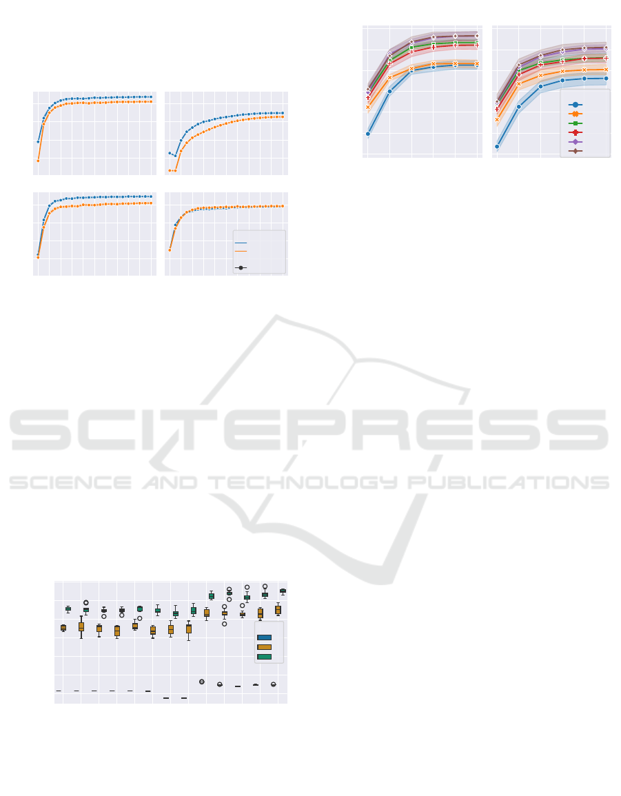
the models’ performance. Figure 3 shows the model

performance on the test set over 20 epochs of training

over 10 runs with different random seeds. The models

were trained and evaluated separately on the original

dataset (in orange) and the preprocessed dataset (in

blue).

Almost all models show better performance on the

preprocessed dataset than on the original one in the

zero-shot setting (Epoch 0; no ﬁne-tuning). This indi-

cates that preprocessing is beneﬁcial even though the

models are not yet adapted to the data domain. Es-

pecially, All-DistilRoBERTa-v1 beneﬁtted from pre-

processing, achieving the highest zero-shot perfor-

mance and creating the highest performance gap be-

tween preprocessed and original datasets. Only All-

MiniLM-L12-v2 was indifferent to preprocessing and

showed identical performance on the original and pre-

processed datasets in the zero-shot setting.

Fine-tuning increased the performance of all mod-

els on both datasets, with most performance gains oc-

curring in the ﬁrst few epochs. Subsequent epochs

still increased performance, albeit not much. Addi-

tionally, no performance degradation was observed,

indicating that the models did not overﬁt the small

sets of labeled data. The highest overall perfor-

mance was achieved by Distiluse-base-multilingual-

cased-v1 on the preprocessed dataset with a Spear-

man’s rank correlation coefﬁcient of 0.8726, mark-

ing a 22% improvement in performance compared to

its zero-shot performance. While almost all models

performed better on the preprocessed dataset than the

original one, this was not the case for All-MiniLM-

L12-v2. It continuously showed similar performance

on both datasets and reached its peak performance on

the original dataset, with a Spearman’s rank correla-

tion coefﬁcient of 0.8460. While only observed with

this model, its invariance regarding preprocessing still

provides an interesting insight. Had its general per-

formance been better, preprocessing could have been

avoided, thus simplifying the whole domain adaption

approach.

All models demonstrated performance improve-

ments, suggesting that with additional ﬁne-tuning,

they could surpass their current peak performance.

However, these performance improvements are ex-

pected to be insigniﬁcant since improvements in the

last few epochs were minimal. Overall, ﬁne-tuning

the pre-trained models on the in-domain datasets

Domain Adaption of a Heterogeneous Textual Dataset for Semantic Similarity Clustering

showed substantial performance improvements for all

models. Most models performed better on the prepro-

cessed dataset, on which the best performance was

achieved.

0.70

0.75

0.80

0.85

Correlation

Model = All-DistilRoBERTa-v1 Model = Sentence-T5-base

0 2 4 6 8 10 12 14 16 18 20

Epoch

0.70

0.75

0.80

0.85

Correlation

Model = Distiluse-base-multilingual-cased-v1

0 2 4 6 8 10 12 14 16 18 20

Epoch

Model = All-MiniLM-L12-v2

Dataset

preprocessed

original

Type

Spearman

Figure 3: Model performance in Spearman’s correlation co-

efﬁcient over 20 training epochs with 10 random seeds per

run.

Preprocessing Ablation. This analysis provides in-

sights into the effects of the individual preprocessing

steps on model performance. The model Distiluse-

base-multilingual-cased-v1 was evaluated after ap-

plying consecutive preprocessing steps, and training

for zero, one, and two epochs on the respective par-

tially preprocessed dataset. This was repeated ten

times with different random seeds. Figure 4 shows

the evaluation performance.

In general, training substantially increased per-

None

Normalize Quotation Marks

Normalize Unicode

Normalize Whitespaces

Remove URLs

Truncate Repeating Characters

Direct Replacements

Split Commas

Replacements

Split Identiﬁers

Lowercase

2nd Replacements

Truncate Whitespaces

Preprocessing Step

0.700

0.725

0.750

0.775

0.800

0.825

0.850

Correlation

Model = Distiluse-base-multilingual-cased-v1

Epoch

Figure 4: Spearman’s correlation coefﬁcient after consec-

utive preprocessing steps for Distiluse-base-multilingual-

cased-v1. The model is evaluated after each preprocessing

step. Each evaluation is run with 10 random seeds.

0 1 2 3 4 5

Epoch

0.60

0.65

0.70

0.75

0.80

0.85

0.90

Correlation

Model:

Distiluse-base-multilingual-cased-v1

0 1 2 3 4 5

Epoch

Model:

All-MiniLM-L12-v2

# Negatives

300

600

900

1200

1500

Figure 5: Spearman’s rank correlation coefﬁcient for

Distiluse-base-multilingual-cased-v1 and All-MiniLM-

L12-v2 for different numbers of negative pairs in the

labeled test set over 5 training epochs. The error bands

show the 95% conﬁdence interval.

formance. Training longer showed performance in-

creases for all preprocessing steps, resulting in im-

proved performance for the entire pipeline. In the

zero-shot setting, the ﬁrst preprocessing steps did not

affect performance. The Direct Replacements step

showed the ﬁrst change in performance, lowering it

under the initial baseline. The subsequent Replace-

ments step then shows a large performance improve-

ment, increasing performance above the initial base-

line. The following preprocessing steps then degrade

performance slightly while still maintaining higher

than baseline performance. With training, the previ-

ously negative effect of the Direct Replacements step

could not be observed. However, the Replacements

step was still responsible for the majority of perfor-

mance improvements. Additionally, some subsequent

preprocessing steps, like Truncate Whitespaces, in-

creased performance slightly.

While some steps degraded performance, espe-

cially in the zero-shot setting, it is important to con-

sider the entire preprocessing pipeline since some

steps act in preparation for subsequent steps. In ad-

dition to improving the performance of the semantic

embedding model, preprocessing aims to generate a

cleaned-up document that can then be used to create

topic representations. Thus, preprocessing steps such

as Normalize Whitespaces may not signiﬁcantly im-

pact performance but remain essential for cleaning up

the document.

Negative Samples. This evaluation determines how

many negative samples are beneﬁcial, justifying the

decision to add K = 1200 negative samples to the la-

beled dataset in Section 5.2.2.

Figure 5 shows the performance of two semantic

embedding models with six different amounts of neg-

ative samples. The labeled dataset was created as de-

DATA 2025 - 14th International Conference on Data Science, Technology and Applications

scribed in Section 5.2.2 but with respectively different

amounts of negative samples for K. The models were

evaluated over ten runs with different random seeds.

Increasing the number of negative samples in-

creased the performance for both models up to about

600 negative samples. After this, performance in-

creases only slightly, with 1200 and 1500 negative

samples showing roughly the same performance. As

a result, K = 1200 was chosen as the number of neg-

ative samples to be added to the labeled dataset.

5.3.2 Topic Model

This section addresses the performance of the whole

combined approach. Objectively evaluating the topic

model is difﬁcult since there does not exist a labeled

in-domain dataset for the extraction of topics and

the creation of their representations. Creating such

a dataset is also extremely difﬁcult since this would

require a complete overview of the topics contained

in the dataset and their respective potential represen-

tations. Therefore, the results of the topic model

were evaluated qualitatively by two in-domain experts

from the industrial plant from which the dataset orig-

inated. These experts are specialists in the domain

of the dataset and participated in the dataset’s cre-

ation. They evaluated the sensibility of the extracted

topics along with their representations by ﬁrst assess-

ing the common theme of all documents assigned to

a topic. Then, if a common theme was present and ﬁt

the topic well, they checked whether unrelated doc-

uments – i.e., outliers – were included. Finally, they

compared the topic’s representations with the theme

of the generated topic.

Following this evaluation outline, a good topic

should comprise a well-deﬁned theme that is present

in all documents assigned to that topic. Multiple

topics within a dataset should show as little overlap

in their respective themes as possible. Additionally,

topic representations should reﬂect that theme in a

concise and clear manner. By the subjective nature

of the underlying evaluation criteria, the whole evalu-

ation in itself is also subjective.

Since the topic model is highly customizable,

changing its parameters can substantially impact the

output. The experts found that one such parameter

is the minimum cluster size of the clustering algo-

rithm. Using a high value resulted in a low number

of topics that were often too coarse to represent in-

dividual semantic themes within the dataset. Using

a lower value resulted in a much higher number of

topics, which were more representative regarding in-

dividual themes and more realistic topics. While, as a

result, this parameter’s value was chosen to be 100, it

is highly dependent on the dataset and the similarity

of documents within it. We recommend starting with

a lower minimum cluster size and increasing it until a

desired topic granularity is reached.

The experts found that topic representations were

mostly representative. The extraction of relevant

topic keywords worked well. However, some of the

topic documents that were chosen to be representative

were rather at the margin of the topic and, therefore,

should not have been regarded as representative. Then

again, the language model-based generation success-

fully produced meaningful topic descriptions.

6 CONCLUSION

This work presents guidelines for developing and

customizing a practically applicable domain-speciﬁc

topic model. The approach consists of two stages:

ﬁrst, an extensive preprocessing pipeline for in-

domain data, followed by ﬁne-tuning an existing

domain-agnostic model on a semi-automatically la-

beled subset of this data. Applying and evaluating

the presented approach on a domain-speciﬁc dataset

showed that combining these two steps led to a sub-

stantial increase in model performance on in-domain

data. Here, the best performing semantic embed-

ding model was Distiluse-base-multilingual-cased-

v1, showing a performance increase of 22% compared

to its zero-shot performance. Based on this domain-

adapted semantic embedding model, topic modeling

is applied.

Since domains can vary widely, the presented ap-

proach should serve as a starting point and a guide-

line. It should not be relied upon as a ﬁxed solution

applicable to any domain.

Throughout the development of the presented ap-

proach, it became apparent that if the underlying

dataset is close to commonly used language, the

advantages of preprocessing may be minimal and,

therefore, not justiﬁable. However, if the underly-

ing dataset is domain-speciﬁc, especially in technical

ﬁelds, beneﬁts from preprocessing can reasonably be

expected.

Future work will concentrate on providing an ob-

jective criterion for the qualitative evaluation of the

topic model. This would help with the automatic op-

timization of topic-modeling approaches and relate

them objectively, providing baseline standards.

REFERENCES

Agirre, E., Cer, D., Diab, M., and Gonzalez-Agirre, A.

(2012). SemEval-2012 task 6: A pilot on seman-

Domain Adaption of a Heterogeneous Textual Dataset for Semantic Similarity Clustering

tic textual similarity. In *SEM 2012, pages 385–393.

ACL.

Angelov, D. (2020). Top2vec: Distributed representations

of topics.

Carbonell, J. and Goldstein, J. (1998). The use of mmr,

diversity-based reranking for reordering documents

and producing summaries. In SIGIR ’98, page

335–336. ACM.

Conneau, A., Khandelwal, K., Goyal, N., Chaudhary, V.,

Wenzek, G., Guzm

an, F., Grave, E., Ott, M., Zettle-

moyer, L., and Stoyanov, V. (2020). Unsupervised

cross-lingual representation learning at scale. In ACL

2020, pages 8440–8451. ACL.

Devlin, J., Chang, M.-W., Lee, K., and Toutanova, K.

(2019). BERT: Pre-training of deep bidirectional

transformers for language understanding. In NAACL

’19, pages 4171–4186. ACL.

Farahani, A., Voghoei, S., Rasheed, K., and Arabnia, H. R.

(2021). A brief review of domain adaptation. In Ad-

vances in Data Science and Information Engineering,

pages 877–894. Springer International Publishing.

Gao, L., Biderman, S., Black, S., Golding, L., Hoppe, T.,

Foster, C., Phang, J., He, H., Thite, A., Nabeshima,

N., Presser, S., and Leahy, C. (2020). The pile: An

800gb dataset of diverse text for language modeling.

Grootendorst, M. (2022). Bertopic: Neural topic modeling

with a class-based tf-idf procedure.

Hinton, G., Vinyals, O., and Dean, J. (2015). Distilling

the knowledge in a neural network. In NIPS Deep

Learning and Representation Learning Workshop.

Howard, J. and Ruder, S. (2018). Universal language model

ﬁne-tuning for text classiﬁcation. In ACL 2018, pages

328–339. ACL.

Jiang, A. Q., Sablayrolles, A., Mensch, A., Bamford,

C., Chaplot, D. S., de las Casas, D., Bressand, F.,

Lengyel, G., Lample, G., Saulnier, L., Lavaud, L. R.,

Lachaux, M.-A., Stock, P., Scao, T. L., Lavril, T.,

Wang, T., Lacroix, T., and Sayed, W. E. (2023). Mis-

tral 7b.

Liu, Y., Ott, M., Goyal, N., Du, J., Joshi, M., Chen, D.,

Levy, O., Lewis, M., Zettlemoyer, L., and Stoyanov,

V. (2019). Roberta: A robustly optimized bert pre-

training approach.

Loshchilov, I. and Hutter, F. (2019). Decoupled weight de-

cay regularization.

McInnes, L., Healy, J., and Astels, S. (2017). hdbscan: Hi-

erarchical density based clustering. JOSS, 2(11):205.

McInnes, L., Healy, J., and Melville, J. (2018). UMAP:

Uniform Manifold Approximation and Projection for

Dimension Reduction. ArXiv e-prints.

McInnes, L., Healy, J., Saul, N., and Grossberger, L. (2018).

Umap: Uniform manifold approximation and projec-

tion. JOSS, 3(29):861.

Mikolov, T., Chen, K., Corrado, G. S., and Dean, J. (2013).

Efﬁcient estimation of word representations in vector

space.

Ni, J., Hernandez Abrego, G., Constant, N., Ma, J., Hall, K.,

Cer, D., and Yang, Y. (2022). Sentence-t5: Scalable

sentence encoders from pre-trained text-to-text mod-

els. In ACL 2022, pages 1864–1874.

Pedregosa, F., Varoquaux, G., Gramfort, A., Michel, V.,

Thirion, B., Grisel, O., Blondel, M., Prettenhofer, P.,

Weiss, R., Dubourg, V., Vanderplas, J., Passos, A.,

Cournapeau, D., Brucher, M., Perrot, M., and Duch-

esnay, E. (2011). Scikit-learn: Machine learning in

Python. JMLR, 12:2825–2830.

Radford, A. and Narasimhan, K. (2018). Improving lan-

guage understanding by generative pre-training.

Radford, A., Wu, J., Child, R., Luan, D., Amodei, D., and

Sutskever, I. (2019). Language models are unsuper-

vised multitask learners.

Raffel, C., Shazeer, N., Roberts, A., Lee, K., Narang, S.,

Matena, M., Zhou, Y., Li, W., and Liu, P. J. (2020).

Exploring the limits of transfer learning with a uniﬁed

text-to-text transformer. JMLR, 21.

Reimers, N., Beyer, P., and Gurevych, I. (2016). Task-

oriented intrinsic evaluation of semantic textual simi-

larity. In COLING 2016, pages 87–96.

Reimers, N. and Gurevych, I. (2019). Sentence-bert: Sen-

tence embeddings using siamese bert-networks. In

EMNLP 2019. ACL.

Reimers, N. and Gurevych, I. (2020). Making monolin-

gual sentence embeddings multilingual using knowl-

edge distillation. In EMNLP 2020, pages 4512–4525.

ACL.

Robertson, S., Walker, S., Jones, S., Hancock-Beaulieu,

M. M., and Gatford, M. (1994). Okapi at trec-3. In

TREC-3, pages 109–126. NIST.

Sanh, V., Debut, L., Chaumond, J., and Wolf, T. (2020).

Distilbert, a distilled version of bert: smaller, faster,

cheaper and lighter.

Sun, B., Feng, J., and Saenko, K. (2016). Return of frus-

tratingly easy domain adaptation. In AAAI’16, page

2058–2065.

Taleb, I., Serhani, M. A., and Dssouli, R. (2018). Big data

quality assessment model for unstructured data. In IIT

2018, pages 69–74.

Thakur, N., Reimers, N., Daxenberger, J., and Gurevych,

I. (2021). Augmented SBERT: Data augmentation

method for improving bi-encoders for pairwise sen-

tence scoring tasks. In NAACL 2021, pages 296–310.

ACL.

Tiedemann, J. and Thottingal, S. (2020). OPUS-MT -

Building open translation services for the World. In

EAMT.

Tunstall, L., Beeching, E., Lambert, N., Rajani, N., Ra-

sul, K., Belkada, Y., Huang, S., von Werra, L., Four-

rier, C., Habib, N., Sarrazin, N., Sanseviero, O., Rush,

A. M., and Wolf, T. (2023). Zephyr: Direct distillation

of lm alignment.

Vaswani, A., Shazeer, N., Parmar, N., Uszkoreit, J., Jones,

L., Gomez, A. N., Kaiser, L., and Polosukhin, I.

(2017). Attention is all you need. In Proceedings of

the 31st NIPS, NIPS’17, pages 6000–6010.

Wang, W., Wei, F., Dong, L., Bao, H., Yang, N., and Zhou,

M. (2020). MiniLM: Deep self-attention distillation

for task-agnostic compression of pre-trained trans-

formers. In Proceedings of the 34th NIPS, NIPS’20.

Wilson, G. and Cook, D. J. (2020). A survey of unsuper-

vised deep domain adaptation. TIST 2020.

DATA 2025 - 14th International Conference on Data Science, Technology and Applications