3D Convolutional Neural Network to Predict the Energy Consumption of

Milling Processes

Christoph Wald, Thomas Jung and Frank Schirmeier

Institute for Data-Optimized Manufacturing (IDF), UAS Kempten, Bahnhofstr. 61, Kempten, Germany

Keywords:

Convolutional Neural Network, Machine Tool, Energy Consumption, 3D Shape Analysis, Prediction.

Abstract:

With increasingly ﬂuctuating energy prices, the energy-ﬂexible operation of electrical consumers, including

machine tools, has recently gained attention. This study aims to predict the energy consumption from the shape

of the volume removed during a time step in milling, generated using a time-discrete simulation environment.

A 3D residual network is used to analyze the voxel representation of these ”removed volumes”. In total, 48

unique combinations of cutting depth and feed rate are recorded on a three-axis mill to evaluate the proposed

model. The results indicate that energy consumption prediction using these shapes is possible.

1 INTRODUCTION

The German energy grid is in a process of transforma-

tion towards renewable energies, aspiring 600 TWh to

be produced from renewable energy sources in 2030

in comparison to 245 TWh in 2022 (Bundesminis-

terium f

ur Wirtschaft und Klimaschutz, 2023). How-

ever, volatile sources such as wind and solar en-

ergy are subject to natural ﬂuctuations. (Popp, 2020)

shows how machine tools can be operated in an

energy-ﬂexible manner, enabling the machining in-

dustry to mitigate these effects by increasing or de-

creasing their power consumption accordingly. To

this end, knowledge about the future energetic behav-

ior of machine tools may be used to support planning

of production processes and to optimize their opera-

tion through the control of individual components.

In this study, we investigate how deep learning on

3D data can be used to predict the energy consump-

tion of machining processes with variable Material

Removal Rate (MRR). Its novelty is the direct appli-

cation of a convolutional neural network (CNN) on

the shape of the removed volume, predicting the en-

ergy that is necessary to remove said shape from the

workpiece.

This paper summarizes and expands upon the re-

sults presented in (Wald, 2024).

https://orcid.org/0009-0002-2842-0376

2 LITERATURE REVIEW

2.1 Energy Prediction Models

On a basic level, a manufacturing process may be de-

scribed as a conversion of input materials and energy

to output materials and waste heat (Gutowski et al.,

2006). One way to describe the energy consumption

of machine tools is the Speciﬁc Energy Consump-

tion (SEC), meaning the energy consumed per ma-

chined volume. In the context of turning processes,

(Li and Kara, 2011) model the SEC as a function

solely based on the MRR, whereas (Li et al., 2013) in-

clude the spindle speed as a further variable to predict

the energy consumption of a milling machine. Instead

of summarizing the energy consumption through a

single formula, (He et al., 2012) use a bottom-up

approach where Numerical Control (NC) commands

(the program code used for machine steering) are ana-

lyzed and the energy consumption of individual com-

ponents is separately modeled and ﬁnally summed up.

Recently, more authors investigate machine learn-

ing methods as an alternative to the aforementioned

SEC models. A prediction can be understood as an

indication of the current power consumption. One

application of such models is presented by (Sossen-

heimer et al., 2020), where a prediction model is used

as virtual measuring point as an alternative to phys-

ically installed sensors. Similarly, (He et al., 2020)

use a 1D-CNN to predict the current power consump-

tion using the current process properties as features,

including feed rate of and load on the X-, Y- and Z-

Wald, C., Jung, T., Schirmeier and F.

3D Convolutional Neural Network to Predict the Energy Consumption of Milling Processes.

DOI: 10.5220/0013457000003967

In Proceedings of the 14th International Conference on Data Science, Technology and Applications (DATA 2025), pages 21-30

ISBN: 978-989-758-758-0; ISSN: 2184-285X

axis, spindle speed and depth of cut.

On the other hand, the prediction may refer to an

unspeciﬁed point in time in the future, based on cur-

rently available knowledge such as NC code. To this

end, (Brillinger et al., 2021) evaluate different types

of decision trees to predict the energy consumed for

each individual line. (Cao et al., 2021) train a separate

neural network for every type of supported command

(G00, G01, etc.) and ﬁnally sum up all results for the

total energy consumption. (Kim et al., 2022) point

out the difﬁculty of recording extensive data sets from

production environments. They use workpiece mate-

rial properties to transfer knowledge about the power

consumption during milling of steel and aluminum

for predictions using titanium. (Schmitt et al., 2024)

compare a total of 13 regression models to predict

the energy consumption based on NC commands. In

their experiments, a neural network ensemble model

with four hidden layers each and a dropout layer per-

formed best. Similarly, we compare four regression

models: Two CNNs, a linear model and a SEC model;

however, our main contribution is to combine these

with a more domain-speciﬁc machining simulation

approach.

2.2 Machining Simulation

In the literature, a broad range of simulation environ-

ments for subtractive manufacturing processes is pre-

sented. They are generally distinguished by their un-

derlying data structure and their application. (Schn

et al., 2021) developed a voxel-based machining sim-

ulation to calculate the material removal in milling

processes. They use the engagement histogram de-

ﬁned by the area of contact between the tool and the

workpiece in combination with a mechanistic model

to predict cutting and friction forces. (Str

obel et al.,

2023) simulate the kinematics and the material re-

moval process based on NC code. Using a network

with two hidden layers, they predict the current sig-

nal of the X-, Y- and Z-axis and the spindle. (Witt

et al., 2019) present a voxel simulation that includes a

hardware-in-the-loop coupling to a real NC unit used

to obtain the cutting forces during machining. These

forces are in turn used to calculate the displacement

of the tool center point.

In line with this earlier work, we use an algorith-

mic (software-only) machining simulation in order to

gain additional insight into the machining process and

to generate more features that can be used in the sub-

sequent machine learning pipeline. These features are

based on the removed volumes that are generated in

each time step of the simulation.

2.3 3D Shape Analysis Using Deep

Learning

For deep learning on 3D data, different representa-

tions such as voxels, point clouds or meshes exist

(Ahmed et al., 2019). To keep the model architectures

simple, our approach is based on a voxel representa-

tion of the removed volumes. For a regression task

like the prediction of energy consumption based on

voxel data, there exist numerous earlier works in the

literature. For instance, (Pfeiffer et al., 2019) use a

3D CNN on a voxelized organ model to estimate the

organ’s internal deformation. Both, input and output

of the network, consist of a voxel model with a reso-

lution of 64

. Similarly, (Han et al., 2022) use a 3D

CNN to assign the amount of solar radiation to each

voxel of a building representation. (Singh and Smith,

2023) predict the energy consumption of buildings

per square meter and year using a hybrid model that

combines a 3D voxel model of the building and ad-

ditional numerical input values that are merged in

the fully connected layers of the network. (Jafrasteh

et al., 2023) present ”DSCNN”, a 3D CNN that esti-

mates the brain volume based on a 128

voxel model

of 3D ultrasound images, outperforming the 3D ver-

sions of AlexNet, ResNet and VGG.

Deep learning on 3D data entails a set of chal-

lenges, including the representation and the compara-

bly high memory consumption. At the same time, op-

portunities to make informed statements about certain

properties of 3D shapes are opened up. Therefore, we

speciﬁcally investigate the application of deep learn-

ing on 3D data in the context of machining using a

3D residual network architecture (He et al., 2015) that

supports 3D voxel models as input and has a single

output neuron to regress the energy consumption.

3 METHOD

3.1 Overview

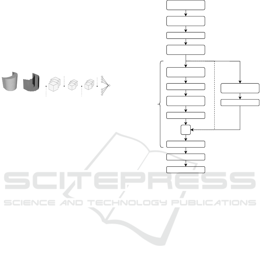
Our pipeline is outlined in Figure 1. We use a sim-

ulation environment to generate ”removed volumes”,

each representing the shape of the material that is be-

ing removed by the interaction of the tool and the

workpiece over a speciﬁed short time interval. The

mesh representation of the removed volume is vox-

elized and serves as input for a subsequent neural net-

work to predict the energy consumption that is mea-

sured and aggregated in said time interval. Our ra-

tionale (cf. (G

otz et al., 2024)) is that the collection

of time-indexed ”removed volumes” contains a very

detailed description of the varying process conditions

DATA 2025 - 14th International Conference on Data Science, Technology and Applications

that contains and extends more traditional measures

like cutting width (a

) and cutting depth (a

The network architecture consists of a convolu-

tional and a max-pool layer, followed by one or more

residual units. Finally, a global-average-pool layer

(used to ﬂatten the 3D structure) leads into the out-

put neuron. In a regression task, this output value is

trained to match the energy consumption associated

with the speciﬁc removed volume used as input for

the neural network.

Mesh Voxel Conv3D Residual Units

MaxPool3D

Energy

GlobalAvgPool3D

Figure 1: Pipeline overview. The cubes represent the fea-

ture blocks after each layer.

The shape of each removed volume implicitly

contains information about the width and depth of the

cut, the geometry of the tool and the current shape of

the workpiece. In a similar manner, also the speed of

the tool relative to the workpiece (the so-called feed

rate) is encoded, because a higher feed rate results in

a more voluminous body that is removed in a given

time interval. For the latter encoding, a constant time

interval between consecutive tool positions evaluated

in the simulation is essential.

Different removed volumes, resulting from differ-

ent cutting parameters, may have the same numeri-

cal value for the total volume as expressed via the

MRR measure. Therefore, our hypothesis is that an-

alyzing the shape of the removed volume should pro-

vide more precise information about the energy con-

sumption than the numerical value for the total vol-

ume of the shape itself. The evaluation of the bene-

ﬁts of the additional information contained in the 3D

shape compared to a simple MRR model forms thus

our main research question.

3.2 Network Architecture

The full network structure is shown in Figure 2, which

is used as baseline architecture for the hyperparame-

ter optimization described in section 5.3. There, the

following parameters of Figure 2 are optimized: The

number of ﬁlters [ﬁlter], the activation function used

[Act], the size of the stride [strides] and the number

of residual units where i is the current residual unit,

beginning with 0. The number of ﬁlters x

per resid-

ual unit is equal to x

= 2

· [ﬁlter]. If dilation is used,

[strides] is representative of the dilation rate. A con-

volutional layer is inserted into the skip connection, if

̸= x

i+1

Input

NxNxNx1

Conv3D

[filter], k=7, s=2

BatchNorm + [Act]

MaxPool3D

k=3, s=2

Conv3D

, k=3, s=[strides]

BatchNorm + [Act]

Conv3D

, k=3, s=1

BatchNorm

GlobalAvgPool3D

Dense (1)

Conv3D

, k=3, s=[strides]

BatchNorm

[Act]

Residual

Unit i

Figure 2: Full network structure.

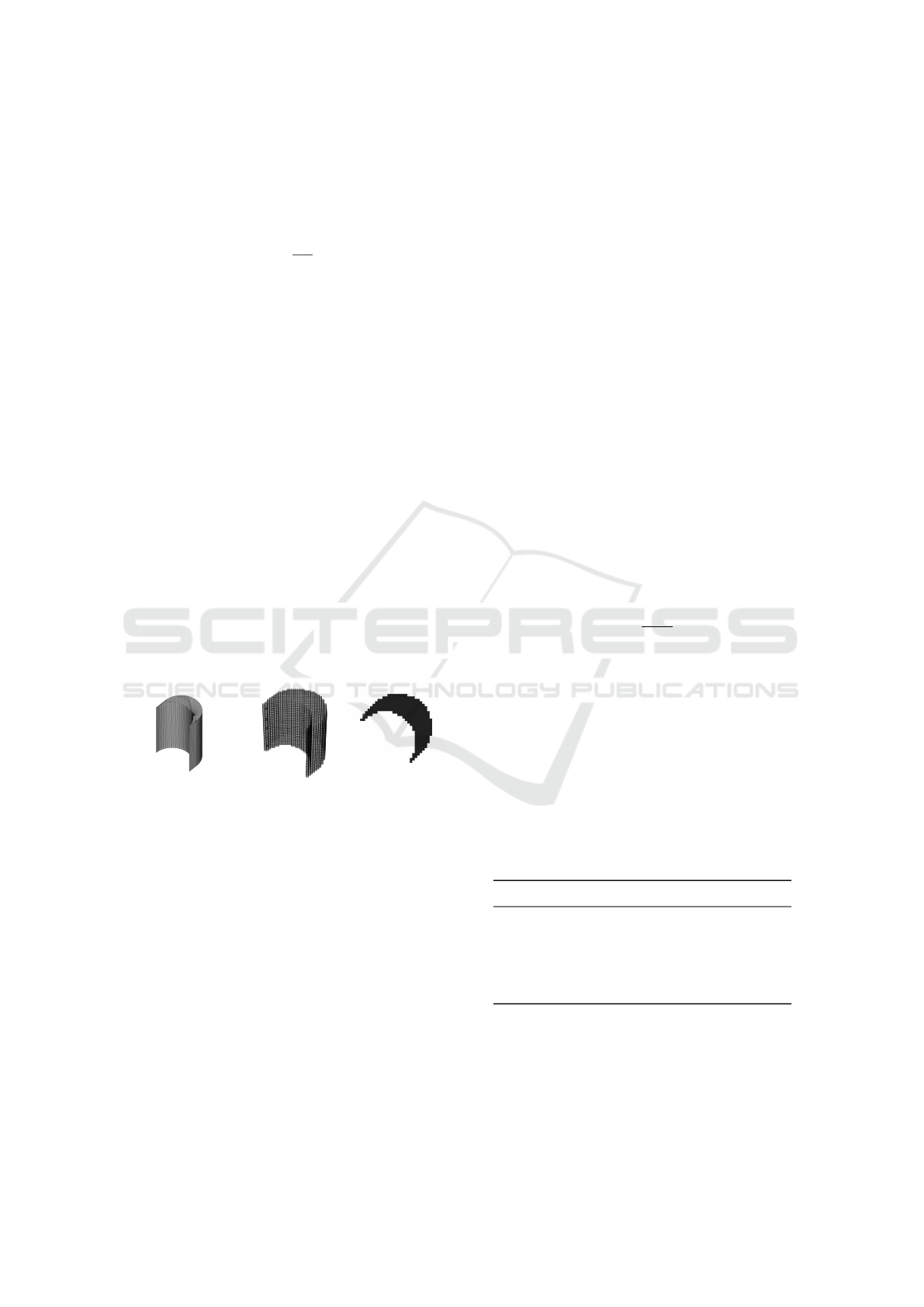
3.3 Removed Volume Voxelization

Voxels are the 3D equivalent to pixels. In their na-

tive representation, each voxel can be accessed with

its indices in the voxel grid. This allows established

2D CNN structures to be adapted to 3D.

Using the python library Trimesh (Dawson-

Haggerty et al., 2019), each removed volume is vox-

elized to be used as input for the proposed 3D CNN.

As a ﬁrst step, each mesh is scaled to ﬁt inside a

cube with a preﬁxed side length. Although maximiz-

ing the occupied space inside this cube would beneﬁt

the preservation of shape details, each mesh is scaled

proportionally to the size of the biggest removed vol-

ume. This is necessary, since information about the

relative differences in the sizes of the removed vol-

ume is a strong indicator of the consumed energy and

therefore cannot be discarded.

Through voxelization, the shape of the removed

volume is then represented by all voxels with a value

of 1, whereas all unoccupied space around the shape

has the value 0. Speciﬁcally, a voxel model may be

hollow (only the voxels representing the surface of the

shape are 1) or ﬁlled (all voxels inside the shape are

also 1). In the experiments presented, the removed

volumes are encoded as ﬁlled voxel models.

3D Convolutional Neural Network to Predict the Energy Consumption of Milling Processes

The level of detail representable by the voxel

model depends on the chosen maximum resolution

V . All voxel models are expanded to a size of V

by padding with 0-voxels and are ﬁnally centered in

this voxel space.

3.4 Simulation Environment

In this study, a simulation environment is used to gen-

erate the removed volume shapes through successive

boolean intersection between tool and workpiece. It

was originally introduced by (Wilkner, 2024) and then

further developed in (G

otz et al., 2024). A total of

three relevant inputs are required:

• The geometry of the tool (height and radius),

• The XYZ-location of the tool according to the cur-

rent NC command or alternatively (as in our ex-

periment) the actual positions as recorded by the

control unit,

• The initial shape and position of the workpiece.

Here, neither the ﬂutes nor the rotation of the tool

is modeled which would lead to a possible extension

of the method. Assuming an end mill, the tool is rep-

resented by a cylinder, which is equivalent to the max-

imum possible volume removed at a particular tool

position.

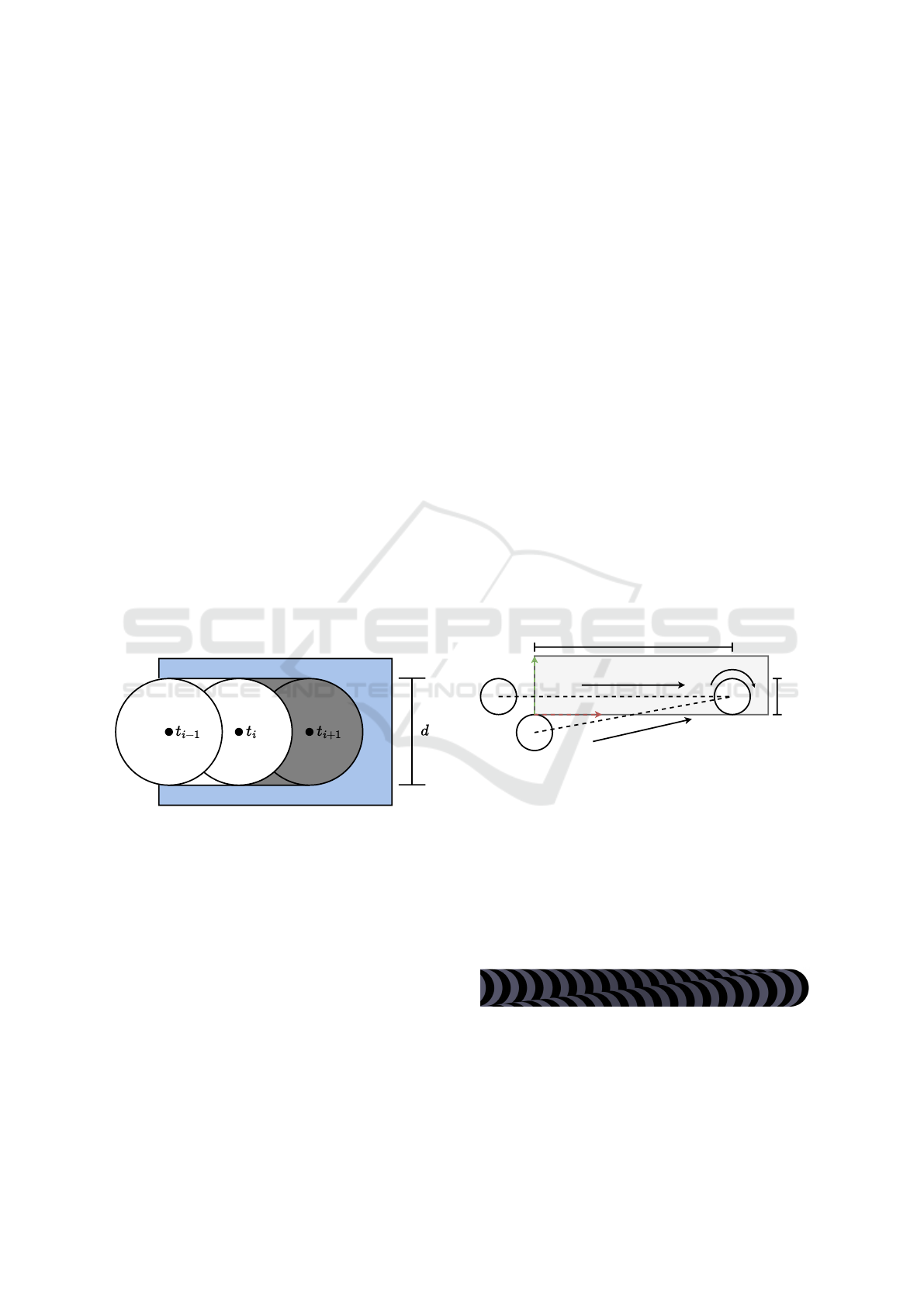
Figure 3: Formation process of a removed volume. The dis-

crete positions of the tool t

{i−1,i,i+1}

, the workpiece (blue)

and the removed volume (grey) are shown.

During simulation, the swept volume (which con-

nects two consecutive tool locations) is continuously

being generated and intersected with the workpiece,

resulting in the removed volume. In Figure 3, the

removed volume is formed by movement of the tool

with diameter d from time step t

until time step t

i+1

The new workpiece geometry is deﬁned by the differ-

ence between workpiece and swept volume.

As shown in Figure 3, the swept volume is nec-

essary to compensate for the discretization of the tool

path. It simulates a smooth and continuous movement

of the tool just like on the real machine tool. Other-

wise, volumes between the individual tool positions

would be missed.

4 EXPERIMENTAL DETAILS

4.1 Experimental Setup

To evaluate our model, we record the power consump-

tion of a three-axis mill. The spindle used is an “AMB

FME-U 1050 DI” with a power rating of 1050 W.

While cutting depth, cutting width and feed are var-

ied, a constant spindle speed of 24,000 rpm is chosen.

The performed combinations of feed rate and cutting

depth are listed in Table 1. An end mill with a di-

ameter of 6 mm and two ﬂutes (Ceratizit Article-No.

500144060) is used to machine aluminum EN AW-

7010 under dry cutting conditions.

The power of the spindle is recorded separately

from the control unit with the connected feed servos.

Therefore, two Janitza CT27-35 current transform-

ers are used in combination with a Janitza UMG604,

from which the measurements are polled via Modbus.

The currently executed NC line and the current loca-

tion of the tool are polled cyclically from the GRBL

controller. Both controller information and measure-

ments are recorded with their respective time stamp

of receipt.

For each combination of feed rate and cutting

depth, two paths are milled as shown in Figure 4.

50 mm

6 mm

First cut

Second cut

Figure 4: Movement of the tool, performed once for each

combination of feed rate and cutting depth.

First, the cutting width is continuously increased

until the tool is fully engaged, moving from (X=0,

Y=-3) to position (X=50, Y=3). For the second cut, a

different start position is chosen (X=-6, Y=3), result-

ing in a continuous decrease of the cutting width (all

units in mm). The Z-position is adjusted accordingly

to achieve the required depth of cut. As shown in Fig-

ure 5, different shapes are generated for each cut.

Figure 5: Visualization of the removed volumes generated

by simulating the process described in Figure 4.

Each performed experiment for the combinations

listed in Table 1 follows the same procedure (see Fig-

ure 6): First, peak power consumption appears dur-

DATA 2025 - 14th International Conference on Data Science, Technology and Applications

Table 1: Number of unique removed volumes per feed rate and cutting depth, using a voxel resolution of 40

Cutting depth a

in mm

Feed rate v

in mm/min 0.25 0.5 0.75 1.0 1.25 1.5 1.75 2.0

∑

50 447 523 524 424 434 475 511 541 3879

120 186 200 220 206 205 223 205 215 1660

190 150 125 132 146 151 132 134 152 1122

260 101 103 95 110 95 105 115 111 835

330 79 87 85 82 84 86 84 87 674

400 75 75 78 78 77 73 77 78 611

∑

1038 1113 1134 1046 1046 1094 1126 1184 8781

ing acceleration of the spindle (A). Next, a “deﬁni-

tion cut” (B) is performed that removes any leftover

material that was not completely removed during the

cuts for the previous combination. Now, the two cuts

described in Figure 4 (C, E) are performed with a fast

repositioning of the spindle in between (D). Finally,

the spindle is stopped until the next experiment be-

gins (F).

Figure 6: Power consumption during the successive steps in

the experiments.

Focusing on the power consumption of the two

performed cuts, a recurrent pattern for all experiments

can be observed. During the ﬁrst cut (C), the power

consumption increases with the width of cut. For the

second cut, the power consumption rapidly increases

from the ﬁrst contact with material and then gradu-

ally decreases along the cut until the ﬁnal position is

reached. As shown in Figure 7, this behavior is con-

sistent for all depths of cut performed in the experi-

ments.

4.2 Data Preparation

As described in section 3.1, the duration between two

consecutive tool positions must be constant to allow

Figure 7: Power consumption of the spindle during interac-

tion of the tool with the workpiece (C and E in Figure 6)

depending on the depth of cut (v

= 400 mm/min).

for a reasonable interpretation of the feed rate by the

deep learning model. Therefore, intervals of length

∆t = 200 ms are generated and the simulation is eval-

uated at multiples of this length only. Since for these

time stamps it is not guaranteed that corresponding

tool positions are available, new intermediate posi-

tions along the tool path are generated at the multi-

ples. The procedure is shown in Figure 8: The tool

position x

is interpolated between the previous (x

)

and the following tool position (x

) in a linear fash-

ion, based on the time elapsed between these two po-

sitions.

Figure 8: Interpolation of new position x

between existing

positions x

and x

3D Convolutional Neural Network to Predict the Energy Consumption of Milling Processes

As expressed in equation 1, the vector ⃗v = x

− x

is formed and multiplied proportionally by the time

elapsed between x

and the new position x

. Finally,

the time-scaled vector ⃗v is added to the previous tool

location x

= x

∆t

·⃗v (1)

The interpolated positions at the end of each in-

terval of duration ∆t are the new consecutive tool lo-

cations used to generate the removed volumes. For

each interval, the total energy consumed is calculated

as the area under the power consumption levels.

5 EVALUATION

5.1 Comparison with Existing Models

The proposed model is compared with the SEC model

by (Diaz et al., 2012) where the energy consumption

in phases with variable MRR was similarly divided

into so called subintervals. Additionally, only the en-

ergy consumption during the removal of material was

predicted which aligns well with the constraints of the

proposed model. Here, the consecutive tool positions

are used as subintervals. The MRR of every subinter-

val, determined by the removed volume, is then used

to predict the consumed energy.

(a) Mesh (b) Voxel (c) 2D projection

Figure 9: Different representations of a removed volume.

Furthermore, an additional 2D CNN is used as a

baseline to evaluate the performance of the 3D CNN.

To do so, the height of the voxel model (Figure 9b)

is encoded as a grayscale image in a top-down view

of the voxel model (Figure 9c). In this speciﬁc case,

no information is lost through the projection since the

height of a removed volume is constant for a speciﬁc

X/Y-position. No further ﬁltering is performed after

the projection, therefore both networks use the same

number of samples. Like the 3D CNN, the 2D CNN is

built upon the baseline architecture of Figure 2 except

that all 3D layers are replaced with their common 2D

versions.

5.2 Training Procedure

The experiments were designed to cover the full range

of low to maximum cutting forces. Here, the goal is

to predict the energy consumption within this known

range, which is reﬂected in the split of the available

data. Therefore, we use a stratiﬁed split on the fea-

tures feed rate and depth of cut to divide all available

removed volumes into 60% training, 20% validation

and 20% test.

Only removed volumes with a volume greater than

0.01 mm

are taken into account. Since the voxeliza-

tion procedure may map two similar removed vol-

umes to the same voxel representation, we analyzed

the number of duplicates in the data set. For 11.97%

of the voxel representations (V = 40) one or more du-

plicates exist. For each group of duplicates, the ab-

solute deviation between minimum and maximum is

calculated. Over all groups, the mean deviation is as

low as 1.01 Ws. We therefore remove all excess du-

plicates to avoid leakage from the training to the vali-

dation and test set.

To train the 3D CNN, the target energy consump-

tion x is standardized in all three splits using the mean

µ and standard deviation σ of the train split as shown

in equation (2).

˜x =

x − µ

(2)

The standardization is reversed for all predictions

˜y as shown in equation (3) to obtain all values y which

can then be used to evaluate the error.

y = ˜y · σ + µ (3)

5.3 Hyperparameter Optimization

We use ”Keras Tuner” (O’Malley et al., 2019) to train

the 3D CNN with a total of 100 random combinations

of the hyperparameters listed in Table 2.

Table 2: Possible hyperparameters.

Hyperparameter Values

Pattern Dilation, Strides

Activation function ReLU, LeakyReLU, ELU

Residual Units 1, 2, 3

Filters 8, 16, 32

Learn rate (η

) 0.005, 0.01, 0.02

The used activation function, the number of resid-

ual units, the ﬁlters per convolutional layer and the

initial learning rate are varied. Furthermore, we inves-

tigate the use of dilation instead of strides following

the results of (Jafrasteh et al., 2023). The full network

DATA 2025 - 14th International Conference on Data Science, Technology and Applications

structure, depending on the chosen hyperparameters,

is shown in Figure 2.

Each model is trained with a batch size of 32

for a maximum of 200 epochs with early stopping

after 20 epochs. Adam is used as optimizer with

an exponentially decaying learning rate scheduling.

The current learning rate in step t is calculated as

η(t) = η

· 0.9

10000

, where η

is the initial learning

rate.

Table 3: Hyperparameters used for evaluation.

Hyperparameter 3D CNN 2D CNN

Pattern Dilation Dilation

Activation function ReLU ReLU

Residual Units 2 2

Filters 16 28

Learn rate (η

) 0.01 0.01

The combination of hyperparameters with the

lowest Mean Squared Error on the validation split is

listed in Table 3. Each model is then retrained for a

maximum of 100 epochs and early stopping after 10

epochs to be used for the evaluations in section 5.5.

For the 2D CNN, the same hyperparameters are

used except for the numbers of ﬁlters, which are ad-

justed to reach a comparable number of trainable pa-

rameters (61.633 for the 3D CNN, 59.977 for the 2D

CNN).

5.4 Error Measurement

We evaluate the models using the Mean Absolute Er-

ror (MAE, equation (4)) and the Root Mean Squared

Error (RMSE, equation (5)) (Riegler, 2017).

MAE(f,t) =

∑

i=1

| f

−t

| (4)

RMSE(f,t) =

∑

i=1

( f

−t

)

(5)

Both quantify the error of the prediction models by

comparing the real energy consumption t with the pre-

dictions f over all N removed volumes in the test set.

A deviation between MAE and RMSE would indicate

the presence of outlier values which would necessitate

further investigations.

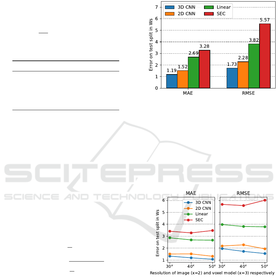
5.5 Results

As explained in section 5.2, a test split was set aside

which is now used to evaluate the different prediction

models. The results shown in Figure 10 are based on

voxel models of size 40

and grayscale images of size

Figure 10: MAE and RMSE on the test split.

The results show that the proposed 3D CNN ar-

chitecture is able to predict the energy consumed by

the machine tool for a given removed volume. While

improvements upon the SEC and linear model were

shown, they are less pronounced in comparison with

the 2D CNN. No signiﬁcant deviation between MAE

and RMSE can be observed for any model. Neither

the deep learning model nor the linear and SEC model

show an excessive number of outliers in their predic-

tions.

Figure 11: Error using different resolutions.

Furthermore, we investigate the impact of using a

lower (30

) and a higher (50

) resolution. For the 2D

model, an image resolution of 30

and 50

are used

respectively. With increasing resolution, the number

of samples in the data set increases as well, since less

duplicate removed volumes exist. For a resolution of

, 8000 unique samples exist. Respectively, 8781

for 40

and 8971 for 50

. The MAE and RMSE, de-

pending on the resolution used, is depicted in Figure

11.

3D Convolutional Neural Network to Predict the Energy Consumption of Milling Processes

The error of the 3D CNN decreases with higher

resolution and is consistently below the error of the

2D CNN. The error of the 2D CNN shows a slight

increase from 30

to 40

but then decreases with a

higher resolution of 50

as well.

Since the linear model is not affected by the reso-

lution the slight decrease of the error can be attributed

to the increased number of samples available during

ﬁtting. However, for the SEC model the opposite can

be observed.

5.6 Discussion

The 2D CNN was included in the experiments to es-

tablish a baseline performance. Since the 3D CNN

outperforms the 2D CNN with a comparable num-

ber of trainable parameters, we conclude that 3D ﬁl-

ters are beneﬁcial in the analysis of the shape of a

removed volume. While the voxel model of the re-

moved volumes could be projected to pixels in this

speciﬁc case, this is not possible for more complicated

shapes and therefore a 2D CNN cannot be employed

anymore. For other tools with a different geometry,

such as ball-end mills, the shapes of the removed vol-

umes are more diverse and we expect a greater beneﬁt

of using a 3D CNN.

Regarding the resolution of the voxel models, the

prediction quality of the CNN models beneﬁts from a

higher resolution. Looking at the progression of the

error of the 3D CNN, the error may further decrease

for resolutions greater than 50

. Since the memory re-

quirement grows cubically with increasing resolution,

a trade-off between resolution and prediction quality

is necessary and could be the objective of future re-

search.

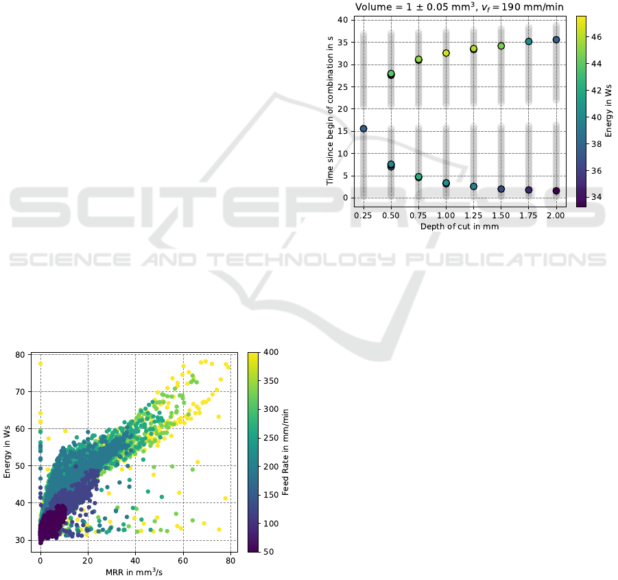
Figure 12: Energy consumption per removed volume as a

function of MRR.

Figure 12 shows that a low feed rate results in

a low MRR which in turn results in a low energy

consumption. For increasing feed rates, the range

of MRR and therefore energy consumption increases.

The correlation between MRR and energy consump-

tion explains the relatively low error of the linear

model. However, Figure 12 also shows that the MRR

on its own is not sufﬁcient to predict the energy con-

sumption.

This becomes particularly clear when comparing

removed volumes that are the result of different cut-

ting conditions but have a similar physical volume as

shown in Figure 13. There, all removed volumes with

a volume of 1 ± 0.05 mm

are highlighted.

Figure 13: Deviation of energy consumption for similar vol-

ume per removed volume.

For different depths of cut, this particular vol-

ume is reached during different times in the exper-

iments. The energy consumption during increasing

MRR (lower half of Figure 13) deviates from the

energy consumption during decreasing MRR (upper

half) within a range of 33 to 47 Ws. With regards to

the results presented, we conclude that the knowledge

different cutting conditions - reﬂected in a different

shape of the removed volume - can be used to make

more accurate predictions about the energy consump-

tion.

Even though the shape of the removed volumes

yields more insight into the process as compared to

the study of the MRR, the energy consumption for

two different shapes may still be identical, just as

with the physical volume. Likewise, the energy con-

sumption for two identical shapes may deviate due to

different spindle speeds or the wear condition of the

tool.

DATA 2025 - 14th International Conference on Data Science, Technology and Applications

6 CONCLUSIONS

This study presents a novel method to predict the

energy consumed by a machine tool during interac-

tion of the tool with the workpiece by combining a

simulation environment and a deep neural network.

The experiments show a mean absolute deviation of

1.19 Ws during each interval of 200 ms. We there-

fore conclude that the shape of a removed volume in-

trinsically contains information that facilitates state-

ments about energy consumption during short peri-

ods of observation. The practical application has two

aspects: First, high-resolution information about the

power consumption may be used to gain insight into

the milling process itself and simulate different NC

codes with different parameters. Second, understand-

ing and predicting the energy consumption of ma-

chine tools is one way to support the energy-ﬂexible

operation of machine tools in an increasingly volatile

energy market. Knowing the load proﬁle ahead of

time may enable optimization of the activity of ma-

chine internal auxiliary units or even across machines.

At the moment, information about the spindle

speed, the wear condition of the tool and the work-

piece material are not incorporated. Since these pa-

rameters vary in real world milling, the model has

to be extended to be able to incorporate their impact

on the predicted energy consumption. Therefore, an

enriched deep learning architecture (e.g. (Singh and

Smith, 2023)) may be used in the future to merge nu-

merical and 3D information for accurate results under

different cutting conditions. Further research may in-

clude different representations of the removed volume

such as point clouds, more complicated shapes of re-

moved volumes and the prediction of the energy con-

sumption of individual components, rather than the

total energy consumption.

ACKNOWLEDGEMENTS

The authors thankfully acknowledge the ﬁnancial

support of the Kopernikus-Project ”SynErgie” (Grant

No. 03SFK3T4-3) by the Federal Ministry of Educa-

tion and Research of Germany (BMBF) and project

supervision by the project management organization

Projekttr

ager J

ulich (PtJ).

REFERENCES

Ahmed, E., Saint, A., Shabayek, A. E. R., Cherenkova,

K., Das, R., Gusev, G., Aouada, D., and Ottersten,

B. (2019). A survey on Deep Learning Advances on

Different 3D Data Representations.

Brillinger, M., Wuwer, M., Abdul Hadi, M., and Haas, F.

(2021). Energy prediction for cnc machining with ma-

chine learning. CIRP Journal of Manufacturing Sci-

ence and Technology, 35:715–723.

Bundesministerium f

ur Wirtschaft und Klimaschutz (2023).

Erneuerbare Energien in Zahlen.

Cao, J., Xia, X., Wang, L., Zhang, Z., and Liu, X. (2021).

A Novel CNC Milling Energy Consumption Predic-

tion Method Based on Program Parsing and Parallel

Neural Network. Sustainability, 13(24).

Dawson-Haggerty et al. (2019). trimesh.

https://trimesh.org/.

Diaz, N., Ninomiya, K., Noble, J., and Dornfeld, D.

(2012). Environmental Impact Characterization of

Milling and Implications for Potential Energy Savings

in Industry. Procedia CIRP, 1:518–523. Fifth CIRP

Conference on High Performance Cutting 2012.

otz, M., Rost, M., Wilkner, D., and Schirmeier, F. (2024).

Unsupervised Segmentation of CNC Milling Sen-

sor Data into Comparable Cutting Conditions. In

Database and Expert Systems Applications: 35th In-

ternational Conference, DEXA 2024, Naples, Italy,

August 26–28, 2024, Proceedings, Part II, page

149–155, Berlin, Heidelberg. Springer-Verlag.

Gutowski, T., Dahmus, J., and Thiriez, A. (2006). Electrical

energy requirements for manufacturing processes. In

13th CIRP international conference on life cycle engi-

neering, volume 31, pages 623–638.

Han, J. M., Choi, E. S., and Malkawi, A. (2022). CoolVox:

Advanced 3D convolutional neural network models

for predicting solar radiation on building facades.

Building Simulation, 15(5):755–768.

He, K., Zhang, X., Ren, S., and Sun, J. (2015). Deep Resid-

ual Learning for Image Recognition.

He, Y., Liu, F., Wu, T., Zhong, F.-P., and Peng, B. (2012).

Analysis and estimation of energy consumption for

numerical control machining. Proceedings of the In-

stitution of Mechanical Engineers, Part B: Journal of

Engineering Manufacture, 226(2):255–266.

He, Y., Wu, P., Li, Y., Wang, Y., Tao, F., and Wang, Y.

(2020). A generic energy prediction model of machine

tools using deep learning algorithms. Applied Energy,

275.

Jafrasteh, B., Lubi

an L

opez, S., and Benavente Fern

andez,

I. (2023). A deep sift convolutional neural networks

for total brain volume estimation from 3D ultrasound

images.

Kim, Y.-M., Shin, S.-J., and Cho, H.-W. (2022). Pre-

dictive Modeling for Machining Power Based on

Multi-source Transfer Learning in Metal Cutting. In-

ternational Journal of Precision Engineering and

Manufacturing-Green Technology, 9(1):107–125.

Li, L., Yan, J., and Xing, Z. (2013). Energy requirements

evaluation of milling machines based on thermal equi-

librium and empirical modelling. Journal of Cleaner

Production, 52:113–121.

Li, W. and Kara, S. (2011). An empirical model for predict-

ing energy consumption of manufacturing processes:

3D Convolutional Neural Network to Predict the Energy Consumption of Milling Processes

a case of turning process. Proceedings of the Institu-

tion of Mechanical Engineers, Part B: Journal of En-

gineering Manufacture, 225(9):1636–1646.

O’Malley, T., Bursztein, E., Long, J., Chollet, F., Jin,

H., Invernizzi, L., et al. (2019). Kerastuner.

https://github.com/keras-team/keras-tuner.

Pfeiffer, M., Riediger, C., Weitz, J., and Speidel, S. (2019).

Learning soft tissue behavior of organs for surgical

navigation with convolutional neural networks. Inter-

national Journal of Computer Assisted Radiology and

Surgery, 14(7):1147–1155.

Popp, R. S.-H. (2020). Energieﬂexible, spanende Werkzeug-

maschinen - Analyse, Bef

ahigung und Erfolgsaus-

sichten. PhD thesis, Technische Universit

at M

unchen.

Riegler, G. E. (2017). Deep Learning for 2.5D and 3D. PhD

thesis, Graz University of Technology.

Schmitt, A.-M., Miller, E., Engelmann, B., Batres, R.,

and Schmitt, J. (2024). G-code evaluation in CNC

milling to predict energy consumption through Ma-

chine Learning. Advances in Industrial and Manufac-

turing Engineering, 8:100140.

Schn

os, F., Hartmann, D., Obst, B., and Glashagen, G.

(2021). GPU accelerated voxel-based machining sim-

ulation. The International Journal of Advanced Man-

ufacturing Technology, 115(1):275–289.

Singh, M. M. and Smith, I. F. C. (2023). Convolutional neu-

ral network to learn building-shape representations for

early-stage energy design. Energy and AI, 14:100293.

Sossenheimer, J., Vetter, O., Abele, E., and Weigold, M.

(2020). Hybrid virtual energy metering points - a low-

cost energy monitoring approach for production sys-

tems based on ofﬂine trained prediction models. Pro-

cedia CIRP, 93:1269–1274. 53rd CIRP Conference

on Manufacturing Systems 2020.

Str

obel, R., Probst, Y., Deucker, S., and Fleischer, J. (2023).

Time Series Prediction for Energy Consumption of

Computer Numerical Control Axes Using Hybrid Ma-

chine Learning Models. Machines, 11(11).

Wald, C. (2024). Deep Learning auf 3D-K

orpern

zur Vorhersage des Energieverbrauchs bei Zerspan-

prozessen. Master’s thesis, Kempten University of

Applied Sciences.

Wilkner, D. (2024). Entwicklung einer performanten Ab-

tragssimulation f

ur Zerspanungsprozesse. Bachelor’s

thesis, Kempten University of Applied Sciences.

Witt, M., Schumann, M., and Klimant, P. (2019). Real-

time machine simulation using cutting force calcula-

tion based on a voxel material removal model. The In-

ternational Journal of Advanced Manufacturing Tech-

nology, 105(5):2321–2328.

DATA 2025 - 14th International Conference on Data Science, Technology and Applications