Research on Manual Carrier Landing Task in High Sea Conditions

XinZe Xu

, Guanxin Hong

and Liang Du

School of Aeronautic Science and Engineering, Beihang University, Beijing, 100191, China

Smart Aviation Center, Hangzhou Innovation Institute of Beihang University, Hangzhou, 311115, China

Keywords: Flight Mechanic, Pilot Model, Carrier Landing Task, Model Predictive Control, Simulation.

Abstract: A model for manual carrier-based aircraft landing missions was established for high sea condition

environments. The model includes pilot, aircraft, deck motion and carrier air wake. The pilot model uses an

intelligent structure, include perception, decision-making and execution modules. The perception module

considers the pilot's perception of unstructured and structured data processes, established through fuzzy

methods and Kalman filtering. The decision-making module is based on MPC (Model Predictive Control)

methods, considering the aircraft pilot's control characteristics based on trend prediction, enabling the

description of the pilot's control strategy under control input and rate constraints. The established pilot model

completed flight simulations in high sea conditions. Simulation results indicate that as sea condition levels

increase, the longitudinal trajectory deviation of manual landings significantly increases, with reduced

correction abilities for deviations caused by ship motion, reflecting the pilot's adaptive adjustment strategy

based on control resource margins under control rate and input constraints. As sea condition levels rise, the

distribution of touchdown point deviations during manual landings increases, posing significant safety risks,

validating that the manual landing model established in this study can be used to analyse the safety of aircraft

carrier landings in complex environments.

1 INTRODUCTION

Aircraft carriers are known as the most dangerous

operating airports in the world, with naval aviators

being the protagonists in this hazardous operating

environment. Currently, manual landing remains the

primary method for aircraft carrier landings. Statistics

show that 80% of accidents involving carrier-based

aircraft occur during the landing process (Haitao &

Yan, 2021; Wang, Jiang, Zhang, & Wen, 2022). In

manual landing mode, naval aviators of carrier-based

aircraft need to control three variables: speed,

altitude, and lateral deviation, requiring a high level

of precision in maintaining control. Providing a

comprehensive description of the control behaviour

of carrier-based aircraft pilots is difficult, hence

practical models that satisfy the closed-loop human-

machine system are typically established. Currently,

there are various practical pilot models available in

the field of carrier-based aircraft, categorized based

on modelling principles into classical control theory

models, physiology models, modern control theory

models, and intelligent models (Xu, Tan, Efremov,

Sun, & Qu, 2017). The classical control theory model

is established based on frequency domain criteria

proposed by McRuer and others. In the early days, the

U.S. military often used quasi-linear models to

describe the pitch channel control behaviour of pilots

during the approach phase of carrier-based aircraft

(D. T. McRuer & Jex, 1967). The physiology model

is based on the structural pilot model proposed by

Hess. Detailed explanations of this modelling

approach can be found in references 5-9. These

models are also based on identification results and are

typically single-channel models based on classical

control theory (Hess, 1980; Hess, 2006; Hess, 2019;

R. A. J. P. o. t. I. o. M. E. Hess, Part G: Journal of

Aerospace Engineering, 2008; M. M. Lone, Ruseno,

& Cooke, 2012). With the widespread application of

artificial intelligence, some scholars have also

introduced intelligent methods to construct model

parameters, extending this model to a wider range of

flight control tasks (Brutch & Moncayo, 2024;

Jakimovska, Pool, van Paassen, & Mulder, 2023).

The two types of models mentioned above mainly

address the description of pilot control behavior for

single-channel flight tasks (such as pitch angle

tracking), but due to their inherent characteristics,

they struggle to describe coupled control channel

operations. NASA reports that as task complexity

Xu, X., Hong, G. and Du, L.

Research on Manual Carrier Landing Task in High Sea Conditions.

DOI: 10.5220/0013432600003970

In Proceedings of the 15th International Conference on Simulation and Modeling Methodologies, Technologies and Applications (SIMULTECH 2025), pages 175-184

ISBN: 978-989-758-759-7; ISSN: 2184-2841

175

increases, models based on frequency domain

identification results may prove insufficient (Baron,

Kleinman, & Levison, 1970; Kleinman, Baron, &

Levison, 1970).When it comes to multi-channel

control, even if it is possible to extend the

construction method of single-channel models to

multiple channels, it is challenging to address the

issue of model structure determination. It also

requires the decoupling of each channel, which limits

the application of quasi-linear models and structural

models in complex conditions involving multiple

inputs and multiple outputs.

Optimal pilot models based on modern control

theory have significant advantages in dealing with

multi-loop control problems. Since these models

describe the pilot's control behavior from the

perspective of overall performance based on optimal

assumptions, strict decoupling is not required (Lone

& Cooke, 2013; D. McRuer, Schmidt, & Dynamics,

1990). The main difference between the optimal pilot

model and the structural model lies in its modeling,

which is not based on frequency domain

identification criteria but on an assumption that aligns

with natural intuition: that human pilot control

behavior is to some extent optimal. The validity of

this assumption has been studied extensively (Roig,

1962). Based on experience, pilots always aim to

maintain a phase margin of 50°-100°for the man-

machine system. In the low frequency range, the

pilot's control behavior is somewhat optimal, aligning

with some theories in optimal control theory (Myers,

Johnston, & McRuer, 1982). Based on the optimal

assumption, discussing the pilot's control behavior

from the perspective of overall performance

optimization becomes feasible. By designing a

reasonable model structure, the optimal model can be

gradually extended to a wider range of flight tasks,

such as the LQR pilot model, MOCM-AE pilot model,

etc. The successful applications of these models have

all demonstrated the validity of extrapolating models

based on the optimal assumption (Davidson &

Schmidt, 1992; Wierenga, 1969).

The ship motion induced by high sea conditions

and complex ship wakes are important environmental

variables affecting the safety of ship landings. A

rising ship wake increases the risk of collision.

Stronger ship wakes and optical guidance motions

caused by heaving and pitching movements further

increase tracking difficulties (optical guidance

typically operates in a line-stabilized form, only able

to counteract ship rotations causing motion in the

optical sphere). This necessitates pilots to focus more

on controlling the overall flight trends. The optimal

assumption is currently the most suitable assumption

for establishing a MIMO human-machine system

pilot model. Therefore, this paper adopts a

constrained MPC method based on the optimal

assumption to establish the pilot model. Within the

constraint range, this model is equivalent to the LQG

pilot model, which has been proven applicable in

describing pilot control behavior. At the constraint

boundaries, by setting reasonable physical constraints,

pilot operations align more with realworld scenarios.

The main innovation of this paper is the

establishment of a pilot model for landing task,

integrating the pilot's predictions and dynamic

constraints during the landing process. Based on the

closed-loop human-machine system established,

which includes the ship motion, aircraft, pilot, and

environment, research on flight safety under high sea

conditions was conducted. This paper investigates the

manual carrier landing task under high sea conditions.

In this section, the research status of this field is

elucidated. The paper describes in the second section

the pilot model established based on the MPC method,

and supplements necessary carrier aircraft, ship

motion, and ship wake engineering models in the

third section to close the human-machine system loop.

Based on the established human-machine system,

simulation experiments of the manual carrier landing

task under high sea conditions are conducted in the

fourth section, discussing the results, and

summarizing the conclusions in the fifth section.

2 PILOT MODEL BASED ON MPC

METHOD

2.1 Overview of Manual Landing Task

The manual landing task of carrier-based aircraft is a

complex task, requiring pilots to manage variables in

three channels: pitch, altitude, and lateral deviation,

based on multiple perceptual information. To

establish a manual landing model for high sea

conditions, it is necessary to have a comprehensive

understanding of carrier landing missions. This

section, based on the description of carrier landing

missions, constructs a conceptual manual landing

model structure: the aircraft captures the desired glide

slope window from a distance behind the carrier. As

shown in Figure 1, guided by FLOLS, the aircraft

aligns with the ideal glide path and successively

completes the landing through a safety window.

Due to the movement of the carrier and the

disturbance caused by the carrier's airflow wake, it is

nearly impossible to maintain the flight path

SIMULTECH 2025 - 15th International Conference on Simulation and Modeling Methodologies, Technologies and Applications

176

accurately. To minimize risks, landing signal officers

are typically stationed on the carrier deck to assist

pilots during landings. LSO are usually experienced

pilots who guide the pilot by predicting aircraft trends

for the next 2-3 seconds and ship movements. They

provide verbal commands like "high" or "low" to help

the pilot adjust their trajectory, which can be seen as

a way of introducing future information into the

guidance process.

In addition to the verbal commands from the LSO,

pilots also obtain the height deviation angle Δ𝑒

through the FLOLS optical guidance system during

the landing process. The literature outlines the

working principles of optical guidance for carrier

landings (Chen, Tan, Qu, & Li, 2018). The optical

guidance system provides feedback on the deviation

angle between the carrier-based aircraft and the ideal

glide path. There are various modelling processes

involved in how pilots handle this guidance

information (Chen et al., 2018; SCHMIDT, 1988).

This article uses the Kalman filtering method to

establish the process by which pilots convert the

deviation angle ∆𝑒 to height deviation ∆𝐻 as they

approach the stern of the carrier. The pilots

continuously self-correct based on observation

results, incorporating observation noise v to simulate

the pilots' observation deviation. The implementation

is as follows: first, establish the state equations for

optical ball displacement and height deviation. The

relationship between the height deviation angle Δ𝑒,

height deviation Δ𝐻, and distance from the carrier

𝑅



is as follows:

Δ𝑒=

∗

Δ𝐻

𝑅



(1)

It can be observed that the value of the deviation

angle is inversely proportional to the distance from

the carrier. By taking X



=

∆















, introducing

system noise w and observation noise v, the state

transition equation for the FLOLS system can be

derived:

𝑋

(

𝑘+1

)

𝐴



(

𝑘

)

+𝑤

𝑍=𝐶



(

𝑘

)

+𝑣

(2)

The pilot's estimate of the height deviation ∆𝐻





can be represented by equation (3), where F is the

Kalman gain, and X





is the estimate state of X



∆𝐻





=𝐴







(

𝑘−1

)

+𝐹∗



𝑍−𝐶



∗𝑋





(

𝑘

)



(3)

This article adopts the structure of intelligent pilot:

perception, decision and execution to establish the

pilot model. The manual approach landing model

structure is shown in Figure 1, where G(s) represents

the pilot's action execution transfer function, and the

perception model is as shown in equations (1-3). The

next section will establish the pilot decision model to

obtain the final actual operational instruction 𝑢



Perception

Information

Pilot

Decision

Model

G(s)

Ship, Aircraft and Environment

Model

Pilot Perception

Model

Decision

Information

Figure 1: Perception, Decision, Action-Based Pilot Model

Structure.

To make the model closely resemble the actual

landing process, this article also designs the following

assumptions to make the pilot model fit human

capabilities to the greatest extent possible. The

specific assumptions are as follows:

1. Throughout the entire process, noise generated

by the pilot's own physiological characteristics

is assumed to be common zero-mean white

noise in nature, with noise within each time

interval being independent. The intensity of the

noise is linearly related to the task load.

2. The pilot will strive to make optimal decisions,

but only decisions within a limited time

interval will conform to the Bellman equation.

3. Regarding the dynamic characteristics of the

aircraft, the pilot has sufficient prior

knowledge for interpretation, and with the

assistance of the landing signal officer, can

roughly estimate the trend of changes in the

next 2-3 seconds. The pilot will not pre-

emptively act in response to unknown

disturbances.

4. The sampling time for the pilot model is 0.02

seconds.

2.2 Pilot Decision Making Models

Based on MPC Methods

The pilot model describes the process in which

pilots make operational decisions based on the

current state and future trends of the carrier-based

aircraft to output the desired operational instruction

𝑢



. Due to the need to minimize overshoot during

the landing process to avoid the risk of colliding

Research on Manual Carrier Landing Task in High Sea Conditions

177

with the carrier, trend prediction has become a key

focus of carrier-based aircraft pilot control

techniques. Pilots are required to smoothly mesh

with the carrier's movements to complete the

landing, which necessitates controlling the trends in

the next 2-3 seconds to counteract the optical ball

fluctuations caused by the carrier's heaving motion.

Considering the unique nature of carrier landing

missions, this article uses prediction and optimality

as two fundamental features and establishes the

pilot's decision model using MPC method.

The MPC method, similar to the LQR pilot model,

is based on optimal hypothesis to calculate the pilot's

gains, while the LQR model is widely used to

describe the pilot's control behaviour (Davidson &

Schmidt, 1992). Additionally, using the MPC method

can address constraint issues, which is crucial during

the landing process. The following sets up a pilot

model based on MPC, assuming the state space model

of the controlled object as:

𝑥(𝑘+1) =

𝐴

𝑥(𝑘)+𝐵𝑢



(k) + 𝐸𝑤

𝑦(𝑘) =𝐶𝑥(𝑘) +𝐷𝑢



(𝑘)

(4)

Where：

𝑥

(

𝑘+𝑃

)

𝐴



𝑥

(

𝑘

)

𝐴



𝐵𝑢



(

𝑘

)

+⋯

+𝐵𝑢



(

𝑘+𝑃−1

)

𝐴



𝐸𝑤

(5)

The recursive predictive model in Equation (5)

represents the pilot's predictive behaviour regarding

the flight state trends, where P is the pilot's prediction

horizon, m is the control horizon, and k is the discrete

step.

After establishing the mathematical model for

the pilot's predictive behaviour, the next step is to

establish explicit constraint equations reflecting the

physical constraints the pilot faces during the carrier

landing process. Constraints are common in the

pilot's working environment. The residual throttle

control resources left in the small perturbation

model established at the conventional operating

point usually range from only 10% to 15%. If hard

constraints are used in modelling, it could

potentially lead to divergence. Therefore, some

studies describe the pilot's control behaviour as a

highly constrained optimal linear controller. This

significantly affects the pilot's decision behaviour,

not only limiting the pilot's control performance but

also introducing intelligent human characteristics

based on control margins.

The advantage of the pilot model established in

this paper is its ability to explicitly handle constraint

issues. By introducing control constraints as

performance conditions into the performance index,

solving the pilot's control behaviour becomes a

planning problem. The control input constraints are

expressed as:

𝑢



(



)

≤𝑢

(

𝑘+𝑖

)

≤𝑢



(



)

(6)

∆𝑈

(

𝑘

)

≝

∆𝑢

(

𝑘

)

∆𝑢

(

𝑘+1

)

⋮

∆𝑢

(

𝑘+𝑚−1

)



(7)

∆𝑌



(

𝑘

)

≝

⎣

⎢

⎡

∆𝑦



(

𝑘+1

𝑘

)

∆𝑦



(

𝑘+2

𝑘

)

⋮

∆𝑦



(

𝑘+𝑝

𝑘

)

⎦

⎥

⎤

(8)

Clearly, the objective function J contains

inequalities, making it impossible to obtain an

analytically optimal pilot gain solution through

solving the Riccati equation. This is a typical

Quadratic Programming (QP) problem. Based on

Assumption 2, it is assumed that the pilot will

optimize the performance function at each sampling

instant.

Physically, the optimal gain represents the pilot's

control strategy that minimizes the overall deviation

of the flight state through a combination of

experience and the pilot's estimation of the flight

trends. By selecting appropriate Q and R values,

inhuman control behaviour can be avoided, typically

requiring state variables other than altitude and lateral

position not to exceed 1. QP problems are a classic

type of optimization problem for which mature

numerical optimization methods exist, making them

well-studied problems. Therefore, transforming the

pilot's decision problem into the standard form of a

QP problem allows for its solution. The standard form

of a QP problem is:

𝑚𝑖𝑛



𝑧



𝐻𝑧 −𝑔



𝑧,Where 𝐶𝑧≥𝑏

(9)

To standardize the predictive equation as in

Equation (8), we have:

𝑧=𝑈(𝑘)

𝐻=𝑆





𝑄



𝑄𝑆



+𝑅



𝑅

𝐺

(

𝑘+1

𝑘

)

=2𝑆





𝑄



𝑄𝐸

(

𝑘+1

𝑘

)

(10)

Therefore, the objective function transforms into:

𝐽



=∆𝑈

(

𝑘

)



𝐻∆𝑈

(

𝑘

)

−𝐺

(

𝑘+1

𝑘

)



∆𝑈

(

𝑘

)

(11)

SIMULTECH 2025 - 15th International Conference on Simulation and Modeling Methodologies, Technologies and Applications

178

Where：

𝐸

(

𝑘+1

)

=𝑅

(

𝑘+1

)

−𝑆



∆𝑥

(

𝑘

)

−𝐼𝑦



(

𝑘

)

−𝑆



∆

𝑑

(12)

𝑆



⎣

⎢

⎡

𝐶𝐴

𝐶𝐴







⋮

𝐶𝐴







⎦

⎥

⎤

, 𝐼=

𝐼

×

𝐼

×

⋮

𝐼

×

, 𝑆



⎣

⎢

⎡

𝐶𝐵

𝐶𝐴



𝐵





⋮

𝐶𝐴



𝐵





⎦

⎥

⎤

𝑆



⎣

⎢

⎡

𝐶𝐵 0 0 … 0

𝐶𝐴



𝐵





𝐶𝐵 0 … 0

⋮⋮⋮⋱⋮

𝐶𝐴



𝐵





𝐶𝐴



𝐵





…… 𝐶𝐵

⋮⋮⋮⋱⋮

𝐶𝐴



𝐵





𝐶𝐴



𝐵





…… 𝐶𝐴



𝐵





⎦

⎥

⎤

Although physical plant constraints are constant,

in the model above, control constraints depend on the

control margin at the current sampling instant.

Therefore, the constraints are time varying. For any

arbitrary time 𝑡



, after discretization, we have:

∆𝑢



(



)

=𝑢



(



)

−𝑢

(

𝑘

)

∆𝑈



(



)

≝

⎣

⎢

⎡

𝑢



(



)

−𝑢

(

𝑘−1

)

𝑢



(



)

−𝑢

(

𝑘

)

⋮

𝑢



(



)

−𝑢

(

𝑘+𝑚−1

)

⎦

⎥

⎤

(13)

Therefore, by considering the form of ∆U(k), the

inequality structure can be obtained as:



−𝐼

𝐼

∆𝑈

(

𝑘

)

≥∆𝑈



(

𝑘

)

(14)

Consequently, we have transformed the pilot's

decision problem into the standard form of a QP

problem. Numerical optimization methods for QP

problems are well established, such as interior point

methods, which can be used for solving. I will not

delve into details here. Once we obtain the pilot gain

𝐾



, we will have established a complete decision-

making model to derive the pilot's desired command

𝑢



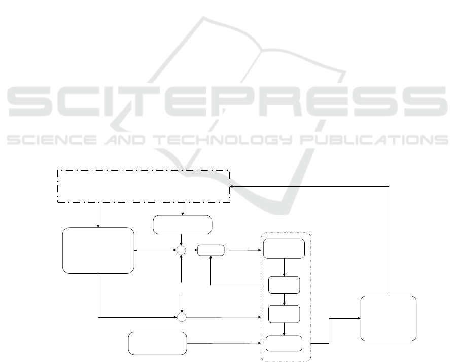
.In conclusion, the overall structure of the pilot

model with constraints added is illustrated in Figure 2.

3 AIRCRAFT SYSTEM

3.1 Aircraft System Model

To study the artificial landing model of carrier-based

aircraft in high sea conditions, it is necessary to

establish a model of the carrier-based aircraft. The

dynamic characteristics of the carrier-based aircraft

model will significantly impact the pilot's landing

performance. In landing tasks, the aerodynamic

effects of the carrier-based aircraft generally satisfy

the assumption of small disturbances, thus a linear

system is used to establish the model of the carrier-

based aircraft (Sweger, 2003). The dynamic equation

is as follows

𝑥=

𝐴

𝑥+𝐵𝑢+𝐸𝑤

=𝐶𝑥+𝐷𝑢



(15)

Fuzzy Perception

System

Altitude Deviation

ObservationΔe

Estimator

Altitude Deviation

EstimateΔH

Lateral Deviation

ObservationΔe

Lateral Deviation

EstimateΔH

Ideal Track Angle

Ship Speed and

Heading

Flight State

ObservationYp

G(s)

Ship, Aircraft and Environment

Model

Position Deviation and

LSO Instructions

Flight State

Prediction

Decision

E(k+1)

Constraint

J(x,u,k)

Optimization

H,G(k)

Figure 2: The Overall Structure of Constrained Predictive Pilot Model.

Research on Manual Carrier Landing Task in High Sea Conditions

179

Where the state variable 𝑥 is:

𝑥=



𝑋,𝑌,𝑍,𝜙,𝜃,𝜑,𝑉,𝛼,𝛽,𝑝,𝑞,𝑟



In the state vector, 𝑋,𝑌,𝑍 represent the

displacements of the carrier-based aircraft in the earth

fixed reference frame, 𝜙,𝜃,𝜑 are the three Euler

angles of the aircraft, 𝑉,𝛼,𝛽 denote the airspeed,

angle of attack, and sideslip angle of the aircraft, and

𝑝,𝑞,𝑟 are the three Euler angular velocities of the

aircraft.

The control input u is:

𝑢=



𝛿



,𝛿



,𝛿



,𝛿





In the control vector, 𝛿



represents the elevator

deflection command, 𝛿



is the aileron deflection

command, 𝛿



is the rudder deflection command, and

𝛿



is the throttle command.

The inner-loop control structure of the aircraft

system is shown in figure 3, aiming to enhance the

flight quality of the system through feedback of 𝛼 and

𝑞 (Chen et al., 2018). Due to the use of pure gain

feedback, the system matrix containing stability

augmentation control can be obtained through linear

transformation. The control model used in this paper

has been somewhat simplified, incorporating the

effects of elevator surfaces and throttle as control rate

constraints into the pilot model. This is done to

analyze the impact of throttle delays and elevator rate

limits on control performance.

Figure 3: Block diagram of the aircraft system.

3.2 Carrier Desire Target Point Model

The position offset of the aircraft is calculated based

on the ideal glide path, with the origin of the ideal

glide path located above the aircraft carrier deck.

Therefore, it is influenced by both the translational

and angular displacements of the ship. In high sea

conditions, the ship will experience more intense

motion, which is a crucial factor affecting landing

safety. Hence, to analyse the impact of high sea

conditions on manual landings, it is necessary to

establish a ship motion model.

The ship motion model in this paper utilizes the

ISSC double parameter spectrum to calculate wave

disturbances, deriving wave interference forces.

Based on the ship's state space response, the time

history curve of ship motion is obtained. The ship

state space is defined as:

𝑥



𝐴



𝑥



+𝐵



𝑢



(16)

The state variable 𝑥



represents:

𝑥





𝑋,𝑌,𝑍,𝜙



,𝜃



,𝜑



,𝑢



,𝑣



,𝑤



,𝑝



,𝑞



,𝑟





The control input 𝑢



represents the wave

disturbance force. After obtaining the ship motion,

the ideal landing point velocity can be derived, as

shown in the following equation:



𝑢



=𝑉



𝑐𝑜𝑠𝜑



𝑣



=𝑉



sin

(

−𝜓



)

𝑠𝑖𝑛𝜑



𝑤



=𝑤



+𝑉



(

𝑠𝑖𝑛𝜃



−𝑠𝑖𝑛𝜙



𝑐𝑜𝑠𝜃



+𝑐𝑜𝑠𝜃



𝑐𝑜𝑠𝜙



)

(17)

𝑢



、𝑣



、𝑤



are the three axis velocities

of the desired touchdown point in the landing

coordinate system, 𝑉



is the speed of the ship, and

𝜓



is the deck angle.

3.3 Carrier Air Wake Model

In high sea conditions, due to the more intense ship

motion and environmental winds, the disturbance

intensity of the ship's wake will also increase

accordingly. The ship's wake consists of four

components, and in the landing coordinate system,

the three axis ship wake field is as follows(Peng, Jin,

& ASTRONAUTICS, 2000):



𝑢



=𝑢



+𝑢



+𝑢



+𝑢



𝑣



=𝑣



+𝑣



𝑤



=𝑤



+𝑤



+𝑤



+𝑤



(18)

In the equation, 𝑢



、𝑣



、𝑤



represent random

free atmospheric turbulence components. 𝑢



、 𝑤



represent steady components of the ship's wake. 𝑢



、

𝑤



represent periodic components of the ship's wake.

𝑢



、 𝑣



、 𝑤



represent random components of the

ship's wake.

4 SIMULATION

In the preceding sections, models for carrier-based

aircraft, ship motion, environmental wind, and pilot

behaviour were established. This paper focuses on sea

conditions 4, 5, and 6 as the research subjects. The

methods for calculating ship wakes and ship motion are

provided in Section 3. Simulation results are shown in

Figure 4. The results indicate that as the sea condition

level increases, the ship's wake motion increases with

the sea condition level, and the corresponding vertical

SIMULTECH 2025 - 15th International Conference on Simulation and Modeling Methodologies, Technologies and Applications

180

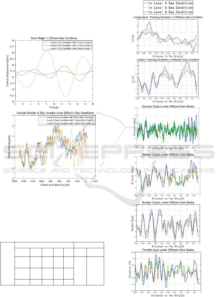
disturbances of the ship's wake flow are enhanced.

Even under sea condition 6 conditions, the ship's wake

motion remains less than ±1.7m, which aligns with the

operational conditions of carrier-based aircraft in the

literature. Therefore, the simulated conditions in this

paper are considered reasonable.

Figure 4: Ship motion and air wake in Level 4-6 sea

condition.

The above environmental conditions serve as

inputs to the simulated study of arrested landings in

high sea conditions. The parameters for the pilot

model are specified in Table 1:

Table 1: Pilot Model Parameters.

Para-

meter

Control Constraints Weight Matrix

Input 𝛿



𝛿



𝛿



𝛿



State Control

Upper

Bound

10.5 25 1 90

𝑄



𝑅



Lower

Bound

-25 -25 -3 75

Vehicle 5 5 0.1 0.1

Conducting simulated arrested landings in high sea

conditions according to the parameters in Table 1,

Figure 5 depicts the behavioural characterization

Figure 5: Pilot Model Output in Level 4,5,6 Sea Conditions.

Research on Manual Carrier Landing Task in High Sea Conditions

181

of pilots in high sea conditions. The simulation results

indicate that the pilot's control magnitude increases in

sea conditions 4, 5, and 6. In sea condition 6, the

ship's wake significantly affects the pilot's landing

operations, showing a trend of oscillation at the ship's

wake, with a notable increase in nonlinear

components in the control command output.

To further conduct a safety analysis of carrier

landings in high sea conditions, repeated simulation

experiments are carried out to study the statistical

characteristics and safety features of arrested landings

in high sea conditions. The repeated simulation

conditions are outlined in Table 2.

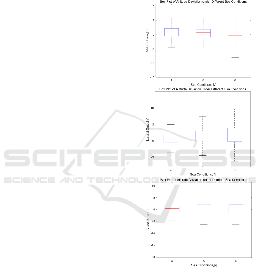
Figure 6 displays box plots of the deviations of

three landing elements in sea conditions 4, 5, and 6.

These elements include altitude deviation, lateral

deviation, and pitch angle deviation, which are the

three main control quantities that pilots need to focus

on during landing tasks. The box plot is a statistical

chart used to display the distribution of data. In box

plot, the data is divided into five parts: the upper

whisker, upper quartile, median, lower quartile, and

lower whisker. The upper whisker represents the

maximum value of the data, while the lower whisker

represents the minimum value. The line in the middle

of the box represents the median (the 50th percentile),

and there are horizontal lines at the top and bottom of

the box representing the upper quartile and lower

quartile, respectively. Box plots also include the

display of outliers, which are values that are typically

far from most data points. Box plots provide a clear

visualization of the data's spread, median, quartiles,

and the distribution of outliers.

Table 2: Simulation Conditions for High Sea condition

Deck Landing.

Name Work Condition Unit

Sea conditions 4，5，6 /

Wind of deck 25 kn

Average wind speed 6，8，14 m/s

Aircraft speed 62 m/s

𝛾

-4 °

Number of Repetitions 45 /

The results indicate that as the sea condition level

increases, the longitudinal deviation in arrested

landings gradually increases. The variance of lateral

deviation remains approximately constant, but the

distribution leans more towards the right side of the

ship's wake. This is because pilots have lower

tolerance for deviations in the longitudinal channel,

prioritizing corrections in that direction. This,

coupled with the longitudinal-lateral coupling, affects

corrections towards the centre, resulting in

insufficient correction for lateral deviations induced

by carrier motion.

Figure 6: Box plot of landing three elements' deviations in

sea condition 4-6.

Figure 7 shows the hook-to-ramp (The vertical

distance between the hook and the ramp when the

aircraft passes through the ramp) clearance of aircraft

passing over the ship's wake in sea conditions 4, 5,

and 6. The hook-to-ramp clearance represents the

safety margin during arrested landings, typically

requiring at least a 4-meter hook-to-ramp distance for

SIMULTECH 2025 - 15th International Conference on Simulation and Modeling Methodologies, Technologies and Applications

182

safety. It can be observed that in sea condition 4,

manual arrested landings can ensure a hook-to-ramp

distance of at least 4 meters, descending from a

position slightly above the ideal trajectory towards

the ship's wake, as described in the literature. In sea

condition 5, the dispersion of hook-to-ramp distances

increases, with a tendency to cross the 4-meter safety

line. In sea condition 6, pilots struggle to maintain a

safe margin of 4 meters for the hook-to-ramp distance,

posing significant safety risks during arrested

landings.

Figure 7: Hook-to-ramp clearance of carrier-based aircraft

in sea conditions 4-6.

5 CONCLUSIONS

This article addresses the modelling issues of carrier

landings task in high sea conditions by establishing

models that include a carrier-based aircraft model,

deck motion model, carrier air wake model, and pilot

model, taking into account the pilot's perception and

decision-making processes. The main conclusions are

as follows:

1. The pilot models based on MPC method under

optimal assumptions, representing a MIMO pilot

model that controls based on the overall state of

the human-machine system. Compared to the

LQR pilot model, the MPC pilot model can

describe the flight techniques where pilots

control based on the trend changes of the ship's

movement and has the structural advantage of

explicitly handling constraints.

2. Simulation results indicate that in high sea

conditions, the longitudinal deviation during

manual arrested landings increases. Due to pilots'

low tolerance for longitudinal deviations and

their high correction priority, corrections for

lateral deviations induced by ship motion are

insufficient, leading to an overall right leaning

lateral deviation. The simulations also

demonstrate that as sea condition levels rise, the

dispersion of hook-to-ramp distances increases

with a tendency to exceed the 4-meter safety line,

posing significant safety risks. This confirms that

the model proposed in this study can be used for

safety analysis of manual carrier landing task in

complex environments.

REFERENCES

Baron, S., Kleinman, D. L., & Levison, W. H. (1970). An

optimal control model of human response part II:

Prediction of human performance in a complex task.

Automatica, 6(3), 371-383. doi:https://doi.org/10.1016/

0005-1098(70)90052-X

Brictson, C. A. (1966). Measures of pilot performance:

Comparative analysis of day and night carrier

recoveries: University of Southern California.

Brutch, S., & Moncayo, H. (2024). Machine Learning

Approach to Estimation of Human-Pilot Model

Parameters. Paper presented at the AIAA SCITECH

2024 Forum.

Chen, C., Tan, W., Qu, X., & Li, H. (2018). A Fuzzy

Human Pilot Model of Longitudinal Control for a

Carrier Landing Task. IEEE Transactions on

Aerospace and Electronic Systems, 54(1), 453-466.

doi:10.1109/TAES.2017.2760779

Davidson, J. B., & Schmidt, D. K. (1992). Modified optimal

control pilot model for compute r-aided design and

analysis. Retrieved from

Haitao, Y., & Yan, L. (2021, 19-22 Nov. 2021). Research

on Key Technologies of Carrier-Based Aircraft

Landing. Paper presented at the 2021 6th International

Conference on Robotics and Automation Engineering

(ICRAE).

Hess, R. A. (1980). Structural Model of the Adaptive

Human Pilot. Journal of Guidance and Control, 3(5),

416-423. doi:10.2514/3.56015

Hess, R. A. (2006). Simplified approach for modelling pilot

pursuit control behaviour in multi-loop flight control

tasks. Proceedings of the Institution of Mechanical

Engineers, Part G: Journal of Aerospace Engineering,

220(2), 85-102.

Hess, R. A. (2019). Analysis of the Aircraft Carrier Landing

Task, Pilot + Augmentation/Automation. IFAC-

PapersOnLine, 51(34), 359-365. doi:https://doi.org/10.

1016/j.ifacol.2019.01.017

Hess, R. A. J. P. o. t. I. o. M. E., Part G: Journal of

Aerospace Engineering. (2008). Obtaining multi-loop

pursuit-control pilot models from computer simulation.

222(2), 189-199.

Jakimovska, N., Pool, D. M., van Paassen, M. M., &

Mulder, M. (2023). Using the Hess Adaptive Pilot

Model for Modeling Human Operator's Control

Adaptations in Pursuit Tracking. Paper presented at the

AIAA SCITECH 2023 Forum.

Research on Manual Carrier Landing Task in High Sea Conditions

183

Kleinman, D. L., Baron, S., & Levison, W. H. (1970). An

optimal control model of human response part I: Theory

and validation. Automatica, 6(3), 357-369.

doi:https://doi.org/10.1016/0005-1098(70)90051-8

Lone, M. M., & Cooke, A. K. J. P. o. t. I. o. M. E., Part G:

Journal of aerospace engineering. (2013). Pilot-model-

in-the-loop simulation environment to study large

aircraft dynamics. 227(3), 555-568.

Lone, M. M., Ruseno, N., & Cooke, A. K. (2012). Towards

understanding effects of non-linear flight control

system elements on inexperienced pilots. The

Aeronautical Journal (1968), 116(1185), 1201-1206.

doi:10.1017/S0001924000007569

McRuer, D., Schmidt, D. K. J. J. o. G., Control,, &

Dynamics. (1990). Pilot-vehicle analysis of multiaxis

tasks. 13(2), 348-355.

McRuer, D. T., & Jex, H. R. (1967). A Review of Quasi-

Linear Pilot Models. IEEE Transactions on Human

Factors in Electronics, HFE-8(3), 231-249.

doi:10.1109/THFE.1967.234304

Myers, T. T., Johnston, D. E., & McRuer, D. J. N. C.-.,

June. (1982). Space shuttle flying qualities and flight

control system assessment study.

Peng, J., Jin, C.-j. J. J.-B. U. O. A., & ASTRONAUTICS.

(2000). Research on the numerical simulation of

aircraft carrier air wake. 26(3; ISSU 103), 340-343.

Roig, R. W. (1962). A comparison between human operator

and optimum linear controller RMS-error performance.

IRE Transactions on human factors in electronics(1),

18-21.

SCHMIDT, D. (1988). Modeling human perception and

estimation of kinematic responses during aircraft

landing. Paper presented at the Guidance, Navigation

and Control Conference.

Sweger, J. F. (2003). Design specifications development for

unmanned aircraft carrier landings: A simulation

approach: US Naval Academy.

Wang, L., Jiang, X., Zhang, Z., & Wen, Z. (2022). Lateral

automatic landing guidance law based on risk-state

model predictive control. ISA Transactions, 128, 611-

623. doi:https://doi.org/10.1016/j.isatra.2021.11.031

Wierenga, R. D. J. I. T. o. M.-M. S. (1969). An evaluation

of a pilot model based on Kalman filtering and optimal

control. 10(4), 108-117.

Xu, S. T., Tan, W. Q., Efremov, A. V., Sun, L. G., & Qu,

X. J. (2017). Review of control models for human pilot

behavior. Annual Reviews in Control, 44, 274-291.

doi:10.1016/j.arcontrol.2017.09.009.

SIMULTECH 2025 - 15th International Conference on Simulation and Modeling Methodologies, Technologies and Applications

184