Energy Consumption Prediction with Uncertainty Quantiﬁcation for

Electric Truck Operations: A Data-Driven Approach

Rik Litjens

1 a

, R

obinson Medina

2 b

, Nikos Avramis

2 c

, Camiel Beckers

2 d

Steven Wilkins

2 e

and Mykola Pechenizkiy

1 f

Department of Mathematics and Computer Science, Eindhoven University of Technology, Eindhoven, the Netherlands

Powertrains Department, TNO, Helmond, the Netherlands

Keywords:

Energy Consumption, Prediction Model, Uncertainty Quantiﬁcation, Battery Electric Vehicle, Fleet

Management, LSTM.

Abstract:

The adoption of electric trucks in commercial applications is growing due the the adoption of zero-emission

zones in large cities. However, the usage of these trucks shows challenges for ﬂeet managers due to their

limited range and uncertain energy usage. Accurately predicting the energy consumption of these vehicles is

crucial for their optimal usage in commercial applications. This work introduces a novel energy consumption

prediction method for electric trucks, based on a data-driven approach. The approach uses a two-stage Long

Short-Term Memory (LSTM) architecture: the ﬁrst stage predicts vehicle speed while the second predicts

energy consumption. For the second stage, two updates to the LSTM encoder are proposed. The ﬁrst im-

proves the energy prediction by splitting the predictions into regenerated and consumed energy, whereas the

second provides a score that quantiﬁes the prediction uncertainty using Student’s t-distribution. Evaluating

the approach using real-world truck-operation data shows that splitting the energy consumption into regener-

ative and consumed components contributes to a 20% reduction of error compared to a state-of-the-art LSTM

model, mainly due to improved prediction accuracy for regenerated energy. Finally, the t-score demonstrates

a 92% reduction of calibration error compared to a Gaussian equivalent. This ensures reliable application in

the design of worst-case planning scenarios, decision thresholds, and probabilistic planning approaches.

1 INTRODUCTION

Governments worldwide are committing to reducing

greenhouse gas emissions and air pollution to pre-

vent climate change and increase living conditions.

A total of 33 countries have pledged to enable 100%

zero-emission medium- and heavy-duty vehicle sales

by 2040 (DriveToZero, 2024). With a 35% increase

in global electric truck sales between 2022 and 2023

and a close to threefold increase within Europe (In-

ternational Energy Agency (IEA), 2024), it is clear

that this is not just a paper reality. In the Nether-

lands, as in many countries worldwide, municipal-

ities have agreed to introduce zero-emission zones

https://orcid.org/0000-0003-0674-1435

https://orcid.org/0009-0001-2214-6153

https://orcid.org/0009-0007-3345-1018

https://orcid.org/0000-0002-3383-1092

https://orcid.org/0000-0001-9498-2321

https://orcid.org/0000-0003-4955-0743

between 2025 and 2030 as part of the 2019 Cli-

mate Agreement (Ministry of Infrastructure and Wa-

ter Management, 2024; Dutch Government, 2019).

The result is that the operation of traditional fossil-

fuel-based transport is partially or fully restricted, in-

creasing the importance of emission-free transporta-

tion.

For large transportation companies, the introduc-

tion of electric medium- to heavy-duty vehicles poses

challenges to ﬂeet managers due to the limited range

of electric trucks, the difﬁculties in estimating how

much energy is needed to carry out a trip (Pelletier,

2019), and the lack of (fast) charging opportunities

along the road. Currently employed solutions intro-

duce inefﬁciencies in the planning process, by for ex-

ample oversizing the vehicle battery needed for a trip,

or providing conservative energy estimations per trip.

An accurate energy consumption prediction would

enable the ﬂeet manager to optimize the routes and

schedules. However, improving prediction accuracy

is often challenging due to uncertainties in the pre-

166

Litjens, R., Medina, R., Avramis, N., Beckers, C., Wilkins, S. and Pechenizkiy, M.

Energy Consumption Prediction with Uncertainty Quantiﬁcation for Electric Truck Operations: A Data-Driven Approach.

DOI: 10.5220/0013362900003941

In Proceedings of the 11th International Conference on Vehicle Technology and Intelligent Transport Systems (VEHITS 2025), pages 166-177

ISBN: 978-989-758-745-0; ISSN: 2184-495X

Table 1: Overview of features and uncertainties for the problem setting.

Available Input Features Measured Features Underlying Uncertainties

Gross combined weight (kg) Front axle speed (km/h) Wind speed and direction

Coordinates (lat, long) Brake pedal position (%) Road conditions

Speed limit (km/h) Acceleration pedal position (%) Driver behaviour

Ambient temperature (deg C) Energy consumption (Wh) Trafﬁc variability

Elevation (m) Powertrain efﬁciency ﬂuctuations

Cornering angle (degrees)

Trafﬁc lights (binary)

dictions, given by variations in the route, e.g., due to

trafﬁc ﬂow, differences in driver behavior, or weather

conditions. Quantifying inherent uncertainties under-

lying the predictions enables uncertainty-aware deci-

sion making in the planning of the vehicles.

Approaches for energy consumption prediction

of electric vehicles can be divided into physics-

based and data-driven approaches. Physics-based ap-

proaches rely on fundamental physical laws to esti-

mate vehicle energy consumption (Yang, 2014; Wu,

2015; Fiori et al., 2016; Fotouhi, 2021). These mod-

els have difﬁculties in capturing variability in energy

prediction because of the above-mentioned uncertain-

ties.

Data-driven approaches leverage large datasets

and machine learning algorithms to capture the en-

ergy dynamics (De Cauwer, 2017; Basso, 2019; Nan,

2022; Pan, 2023). The latter have garnered increas-

ing attention and adoption over the past decade due

to their ability to learn relations without the need for

the direct speciﬁcation of vehicle dynamics (Chen,

2021b) and the increasing amount of available data as

a whole. This work focuses on data-driven models as

they have the potential of capturing the uncertainties

in the energy estimations, while still combining in-

sights from the physics-based modeling approaches.

Data-driven state-of-the-art approaches use a

two-stage model architecture, where the speed proﬁle

and the energy consumption are predicted using

Long Short-Term Memory (LSTM) models (Nan,

2022; Chen, 2021a; Petkevicius, 2021; Feng, 2024).

However, this technique blindly applies the data-

driven approach, where no insights are taken from

the application domain, i.e., the physics behind the

vehicle dynamics. Some works have touched upon

the topic of uncertainty quantiﬁcation (Petkevicius,

2021; Thorgeirsson, 2021) by evaluating uncertainty

scores as a Gaussian random variable. However, the

uncertainty score in (Petkevicius, 2021) produces

calibration intervals that often do not contain the

true values. To the best of the authors’ knowledge,

no strategy available in the literature leverages the

extensive physics knowledge of the electric vehicle

to produce better predictions and quantify the uncer-

tainty in the energy prediction of an electric vehicle

reliably.

The contributions of this paper build upon the

two-stage predictors from the presented literature.

This work improves the second stage (energy

prediction) by:

1. providing a novel architecture that takes into ac-

count the physics of the vehicle, so that regenera-

tive and consumed energy are modeled separately

(LSTM-Decom);

2. introducing the Long Short-Term Memory -

Student-t Mean-Variance (LSTM-TMV) method

that provides uncertainty scores. The method is

based on a Student’s t-distribution which outper-

forms the state-of-the-art Gaussian method.

This paper is organized as follows. Section 2 de-

scribes the speciﬁc setting for which the models are

designed and evaluated. Section 3 describes the pre-

diction architecture and models in it. In Section 4,

the approaches relating to uncertainty scores are de-

scribed. Section 5 presents the results evaluated in a

real data set of an electric truck. Section 6 closes the

paper with conclusions and future work.

2 PROBLEM STATEMENT

This work focuses on the setting where electric trucks

transport goods from a Distribution Centre (DC) to

one or more supermarkets. Each truck must drive var-

ious routes to ensure all supermarkets remain stocked

and return to the DC or a nearby charging station af-

terward. Each part of the route between a DC and/or a

supermarket is considered a “Trip”. The challenge is

to predict the energy consumption of upcoming trips,

using the data features available before departure.

Table 1 describes the available features for the

considered setting. Many of these features are ac-

cessible before the driving phase and are either de-

termined as part of the operating plan (weight and

Energy Consumption Prediction with Uncertainty Quantiﬁcation for Electric Truck Operations: A Data-Driven Approach

167

route) or retrieved through external information sys-

tems (e.g., APIs). The remaining features, which can-

not simply be retrieved before a trip, are found in the

second column of Table 1. They cannot be used as

predictors: instead, they are used for model training

purposes or to analyse the results. The third column

of Table 1 indicates inﬂuencing factors that are infea-

sible to (precisely) measure or forecast and introduce

uncertainty underlying each prediction. Trip data is

available for two trucks of the same model over the

course of two years (2020 and 2021).

The target of this research is to predict the total

amount of battery energy e

consumed in each trip i,

measured in watt-hours (Wh), and quantify the com-

bined magnitude of the underlying uncertainties with

an uncertainty score.

3 METHODOLOGY

The method proposed in this paper builds on the start-

of-the-art data-driven methods for energy consump-

tion prediction and hence includes a two-stage archi-

tecture with the segmentation of the trips (De Cauwer,

2017). To do so, in Section 3.1, trips are divided into

smaller segments, then, in Section 3.2, the speed is

predicted for these segments and, ﬁnally, the energy

consumption is estimated.

3.1 Trip Segmentation

The trips are segmented to capture the local driving

conditions and road variations that directly impact

energy consumption, as well as to provide a consis-

tent input size to the machine learning models. It

is assumed that there are no long-term dependencies

between data points within the trip, as driving be-

haviour or events in the past generally only inﬂuence

the current energy consumption when they occurred

recently. This gives the possibility of segmenting the

trips into smaller sub-sequences. Furthermore, this

structure allows the model to learn from segments

on a more ﬁne-grained level, enabling generalization

across trips. Note that the prediction targets have been

transferred from trip- to segment-level, with each seg-

ment j in trip i having its energy consumption predic-

tion target e

i, j

Equation 1 formalizes the segmented dataset D

with N trips.

(i)

= ((X

i,1

),...,(X

i, j

),...,(X

i,N

))

∀i ∈ {1, . . . , N}.

(1)

Here, X

i, j

represents the sequence of features mea-

sured in segment j of trip i, and e

i, j

is the measured

energy. The predicted energy on the segment level is

summed as ˆe

∑

j=1

ˆe

i, j

, where N

is the amount of

segments in trip i and ˆe

i, j

is the predicted energy for

segment j in trip i.

Two methods for segmentation are used in the

model pipeline:

1. Distance Segmenter. The ﬁrst segmentation

method splits the trips into segments of equal dis-

tance S, with a single data point every ∆s me-

ters. ∆s is deﬁned in such a way that its value

represents a forecasting granularity that can be

achieved before trips.

This method is used for the speed prediction stage,

as time-based methods are unavailable before ve-

hicle speed along the route is known.

2. Change Segmenter. The second method is based

on the elapsed time within a trip and route char-

acteristics: First, trips are split into segments

of T seconds. The choice of T is based on a

trade-off between the size of the input segments

and the amount of context needed to predict the

energy consumption accurately. After this step,

the method is extended with additional segment

“splits” to make the segmentation occur at more

natural points. The technique leverages a subset

of input data features that describe the route ahead

(trafﬁc lights, maximum speed changes, turns);

each time such an “event” occurs, the trip is split

into a new segment.

This method is used for the energy consumption

stage, as the relation between power and energy

consumption depends on time, making the seg-

mentation method more aligned with the physical

process.

3.2 Sequential Modeling Architecture

While segmentation narrows the scope of the predic-

tion problem, modular decomposition allows the in-

troduction of more domain knowledge into the design

of the model pipeline. As acceleration and speed are

inﬂuential features in the dataset for predicting energy

consumption and they are available as measurements,

it is beneﬁcial to create a separate model to predict

these features, instead of relating the inputs to the

energy consumption directly. The results are subse-

quently passed to the energy consumption estimation

stage. This makes the design of the energy consump-

tion estimation model independent of the design of

the speed proﬁle predictor.

VEHITS 2025 - 11th International Conference on Vehicle Technology and Intelligent Transport Systems

168

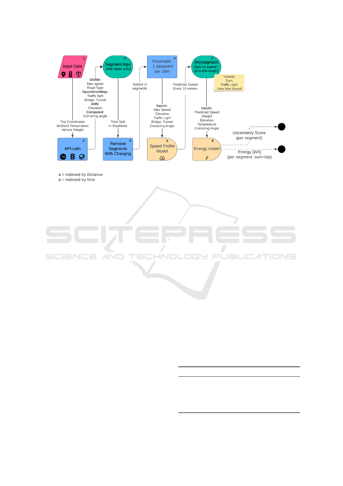
Figure 1: Full evaluation pipeline of the two-stage architecture (uncertainty scores indicated with a dashed line, to indi-

cate they are only present for the uncertainty-aware models). The pink block represents a dataset, the blue boxes indicate

(pre-)processing steps, and the green ovals indicate segmentation steps. Online API’s include Open Source Routing Mahcine

(OSRM), OpenStreetMap, and ‘Algemeen Hoogtebestand Nederland’ (AHN). Finally, the yellow ﬁgures indicate data-driven

prediction models and a black dot represents an output.

Formalizing this structure, one can see the seg-

ment predictor function f as a composite function

consisting of speed proﬁle predictor g and energy con-

sumption estimator h:

f (X

i, j

) = h (g (X

i, j

)) for all trips i and segments j,

(2)

where function f : R

i, j

×d

→ R for d input features

and T

i, j

data points in the input segments.

3.3 Speed Proﬁle Prediction

The ﬁrst stage of the model aims to predict the speed

for upcoming trips. The historical measured speed

data can be used as prediction targets during the train-

ing process of the speed proﬁle prediction model. Im-

plementing the speed predictor requires a sequence-

to-sequence model (i.e., a model that predicts a se-

quence based on one or more input sequences), such

that a single speed prediction is given for each in-

put data point. In this work, speed proﬁles are pre-

dicted for a generic driver, as driver identiﬁers were

not present in the input dataset.

Recurrent Neural Network (RNN) models are a

class of sequence-to-sequence models that can learn

short- to medium-distance dependencies between the

inputs. This aligns with the real-world dependency

structure of driving behaviour. Speciﬁcally, the

model used for this research is a LSTM model,

which is an improvement over the original recurrent

neural network that allows learning over longer input

sequences. The input features and the target feature

are given in Table 2. The initial speed of the segment

is provided during the training process and replaced

with the last prediction of the previous segment

during trip-level predictions.

The model architecture consists of a bidirectional

LSTM module, capturing both past and future speed

proﬁle indicators. An intuitive example of why this

is needed arises when one considers upcoming trafﬁc

events or road features, such as trafﬁc lights. The

speed proﬁle predictor has to account for these before

the vehicle passes the light itself. A stacked 2-layer

setup is used to allow more reﬁned processing of

the sequence. Each LSTM output is passed through

a series of fully connected neural network decoder

layers to produce a sequence of predictions.

Table 2: Input and target features for the LSTM speed pre-

diction model. Inputs and predictions are given on a 1Hz

basis.

Input Features Target Feature

Speed limit (km/h) Speed (km/h)

Elevation (m)

Trafﬁc lights (binary)

Cornering angle (degrees)

Initial speed in segment (km/h)

Energy Consumption Prediction with Uncertainty Quantiﬁcation for Electric Truck Operations: A Data-Driven Approach

169

Figure 2: LSTM encoder architecture. The input sequence

is encoded before being passed to a series of fully connected

(FC) layers that estimate the energy consumption.

Table 3: Input and target features for the LSTM encoder

energy consumption model. Input is given on a 1Hz basis,

predictions on segment level.

Input Features Target Feature

Speed (km/h) Energy (Wh)

Weight (kg)

Elevation (m)

Ambient Temperature (deg C)

Cornering angle (degrees)

3.4 Energy Consumption Estimation

The subsequent step involves developing a model for

estimating energy consumption itself. The training of

this model is done independently and involves true

speed measurements. Even though the proposed ar-

chitecture, where second-by-second data within the

segments is given as an input sequence, is not found

in the literature, the use of LSTM components is

widespread in this and other application domains.

Therefore, the state-of-the-art model is the LSTM en-

coder architecture.

The model uses the entire input sequence X

i, j

predict the energy consumption and produces a sin-

gle scalar output per segment; the input features are

described in Table 3. The input is then processed by

two stacked LSTM layers, keeping track of two hid-

den states throughout the process (see Figure 2). At

the end of the input sequence, the hidden state of the

top layer can be seen as a high-level encoding of the

entire input sequence. This encoding is given as input

for a series of fully connected layers that produce an

energy prediction.

This setup assumes a ﬁxed sequence length for

each segment. However, the input segments have

varying durations as the Change Segmenter uses

events to split the segments. Therefore, the segments

are padded to have equal length.

Evaluations of the performance of the LSTM

encoder model show that the prediction of the

amount of regenerative energy as a result of regen-

Figure 3: Proposed adaptation on energy consumption

pipeline. The entire preprocessing remains the same but

two models are trained to predict positive and negative con-

sumption components.

erative braking is the main source of error, as seen

in Figure 8. Regenerative braking is a technology in

electric vehicles that allows them to recover part of

the energy typically lost during braking and redirect

it back to the battery. The braking energy recovery is

deﬁned within each segment as in Equation 3:

regen,i, j

P(t) · 1

{P(t)<0}

dt, (3)

where e

regen,i, j

represents the total recovered energy

within segment j in trip i, P(t) · 1

{P(t)<0}

indicates

only negative power measurements are summed, and

and t

denote the start and end times of the segment.

Similarly, the consumed energy e

consume,i, j

is deﬁned

by integrating over all positive power values.

The proposed novel architecture builds on the idea

that a different relation between the input features and

energy regeneration exists compared to their relation

to energy consumption. (Fiori et al., 2016; Chen,

2021a) implemented this idea by training separate

models for deceleration and acceleration and swap-

ping between them during inference, as in their setting

the actual acceleration state was always known. In

practice, exact acceleration states often are unknown.

Furthermore, knowing the precise acceleration state

is not required in the two-stage segmented model, as

predictions are performed on the segment level. Each

segment contains both energy regeneration and con-

sumption in varying proportions. The training process

of this model is visualized in Figure 3.

A new method called LSTM-Decom is intro-

duced, where two separate models are created that are

tasked with predicting the regenerative energy e

regen

and consumed energy e

consume

within a segment, re-

spectively. This decomposition allows more control

over the design of each model and its training process.

An important design decision for the regenerative

model is the use of balanced sampling of the training

set. When the input data largely consists of segments

with little to no regenerative energy, which is com-

mon, the training process is hindered. To implement

the balanced sampler, the training set is split into two

groups: the ﬁrst containing segments with more than

VEHITS 2025 - 11th International Conference on Vehicle Technology and Intelligent Transport Systems

170

a minimum threshold of regenerative energy, and the

second group containing the rest. Balanced sampling

is used to undersample from the majority group (i.e.

the group containing segments with little regenerative

energy). For example, consider that there are N

regen

segments with more than 100 W h energy regenera-

tion. Then, all N

regen

high regenerating segments and

only ⌊N

regen

/3⌋ other segments are used as a training

set for the energy regeneration model. Besides reduc-

ing the size of the training set to allow for faster train-

ing, the balanced data set enables a more thorough

understanding of energy regeneration.

4 UNCERTAINTY

QUANTIFICATION

Even after the proposed model improvement, other

sources of error remain, stemming from uncertainties

in the input data. To address these errors, a different

perspective on model error is useful. Let us deﬁne the

prediction error with the equation

i, j

= h

i, j

) + ε

i, j

for all i, (4)

where h

is the energy consumption model trained on

a dataset D with uncertainties. Viewing ε

i, j

as a real-

ization of a random variable allows us to account for

the inherent uncertainty in the predictions. The aim is

to use this new perspective to introduce an additional

uncertainty score that describes this error distribution.

An uncertainty score in energy consumption pre-

dictions allows ﬂeet managers to have a certain level

of conﬁdence in these estimates, helping them an-

ticipate potential variations in energy needs for the

vehicles. Decisions that can be made using this

score range from the creation of prediction intervals,

to worst-case scenarios or the deﬁnition of decision

thresholds, where the predicted value is only trusted

when the accompanying uncertainty is low enough.

The uncertainty score is, therefore, expected to fol-

low the properties described in Deﬁnition 1.

Remark 1. Expected Properties from an Uncer-

tainty Score Energy Prediction

Two properties are expected from an uncertainty

score:

1. A low uncertainty score should correlate with low

prediction errors. A ﬂeet manager should be able

to place trust in predictions made with high cer-

tainty.

2. The uncertainty score should be low when possi-

ble. When the model indicates high levels of un-

certainty for all predictions, it is impossible to act

on it.

Another application of the uncertainty scores entails

a probabilistic approach. Consider, for example, a

planning application based on probabilities of a truck

being able to complete a segment or trip with a cer-

tain amount of energy E. This involves calculating

P(e

i, j

< E). To do so, a point-prediction is made us-

ing input X

i, j

, after which a deﬁciency or surplus is

found with respect to E, denoted by E = h(X

i, j

) +

∆

E,i,j

. For the uncertainty-aware models, the theo-

retical cumulative distribution function (CDF) can be

used to derive this desired probability (see Section 4.2

for a concrete example).

4.1 Gaussian Distribution Method

The state-of-the-art methods assume a zero-mean

Gaussian distribution for the model error, where the

variance is different for each ε

i, j

, i.e.,

i, j

∼ N (0,Var

i, j

)) (5)

with Var

i, j

) as the predicted error variance for in-

put segment j in trip i. The upgrades needed to the

LSTM encoder architecture are shown in Figure 4. As

both the distribution mean and variance are predicted,

the model is called the Gaussian Mean-variance Pre-

dictor (GMP).

4.2 Proposed Student’s t-distribution

Method

This work introduces a novel approach leveraging

Student’s t-distribution with ν degrees of freedom

i, j

∼ t

(0,Var

i, j

)). (6)

The t-distribution is a probability distribution used

in statistics to estimate population parameters when

the sample size is small or the population standard

deviation is unknown. It features heavier tails com-

pared to the normal distribution, reﬂecting the in-

creased variability typically present in smaller sam-

ple sizes. To facilitate the learning process within the

LSTM framework, let us derive from the likelihood

function L

of the Student’s t-distribution with mean

0 and ν degrees of freedom, the Student’s t Negative

Log-Likelihood (TNLL) as

Loss(ε

i, j

,Var

i, j

)) = − log L

(Var

i, j

) | ε

i, j

)

log(Var

i, j

))

ν + 1

log

1 +

i, j

νVar

i, j

)

+ constant, (7)

Energy Consumption Prediction with Uncertainty Quantiﬁcation for Electric Truck Operations: A Data-Driven Approach

171

Figure 4: LSTM encoder architecture with uncertainty

quantiﬁcation. The top branch predicts energy consump-

tion, while the bottom branch produces an uncertainty

score.

where L indicates the loss function. As the loss func-

tion is purely used for comparison, the constant is

irrelevant and removed in the implementation of the

loss function. The cumulative distribution function

for the Student’s t-distribution, used for the proba-

bilistic use case, is:

P(e

i, j

< E) = P(ε

i, j

< ∆

E,i,j

)

= I





, with z =

ν +

∆

E,i, j

Var(X

i, j

)

(8)

where e

i, j

is the true energy consumption and E

an arbitrary reference value for energy consumption.

(a,b) is the regularized incomplete beta function.

The neural network design is equal to that of the

Gaussian mean-variance setup, as seen in Figure 4.

The core difference is the custom PyTorch loss func-

tion incorporating the TNLL loss function. The re-

sulting t mean-variance predictor is named LSTM-

TMV.

4.3 Performance Metrics

The desired properties for the uncertainty score, as

listed earlier in Deﬁnition 1, are translated to two con-

crete metrics:

1. Calibration: This metric captures how often a

predicted value is inside the bounds of a pre-

diction interval. For uncertainty-aware models,

(1−α) prediction intervals are constructed, where

α represents the signiﬁcance level. This statisti-

cal quantity reﬂects the fault tolerance by allow-

ing up to α probability of the true value falling

outside the prediction interval. The intervals can

either be one-sided (to aid in creating a worst-case

scenario upper bound or lower bound) or two-

sided, in which case both a lower bound and upper

bound are present. The percentage of predicted

trips whose true value falls within this predicted

interval indicates the calibration. Theoretically,

this rate should equal 1 − α. Let us therefore de-

ﬁne scores where the rate is 1 − α or higher as

well-calibrated. This metric captures that a “low

uncertainty corresponds to low error”, at least for

(1−α)% of the predictions. When the uncertainty

is lower, the interval is smaller, leaving less room

for error. For example: if the prediction intervals

for 95 out of 100 test trips contain the true value

and α was chosen to be ≥ 0.05, the model is well-

calibrated.

2. Sharpness: This metric captures how far the pre-

dicted value is from the actual value. In principle,

assigning a high uncertainty score to each predic-

tion leads to a high calibration value. This behav-

ior is unwanted. Therefore, we score the adap-

tivity/tightness of the uncertainty score by gener-

ating prediction intervals. The distance between

the true energy consumption value for a trip and

the bounds on the prediction interval deﬁnes the

value for this metric. To give an example: if a trip

has an energy consumption of 50 kWh and the up-

per bound is predicted as 55 kWh, the sharpness

is 10%.

Note that the uncertainty scores are predicted on seg-

ment level, whereas the predictions should be avail-

able on trip level. Simply adding the predicted vari-

ances produces faulty trip-level scores due to the pres-

ence of covariances between individual segments in a

trip. To face this issue, a correlation coefﬁcient ρ is

introduced. The error covariances between segment j

and k in trip i are determined using:

Cov

j,k

= ρ

Var

i, j

)Var

i,k

) (9)

5 RESULTS AND ANALYSES

This section presents how the models described in

Section 3.4 and 4 are trained on a vehicle dataset. To

do so, Section 5.1 presents a motivational case study,

Section 5.2 shows the results for the novel energy con-

sumption model design, and Section 5.3 for the un-

certainty score results. The speed proﬁle predictor re-

sults are important to understand the results of the full

prediction pipeline. Hence, Section 5.4 shows these

results before Section 5.5 describes the full prediction

pipeline results.

5.1 Use Case Description and Model

Training

A dataset is available containing data collected over

two years on two trucks: Truck #1 and Truck #2. Two

test sets are used to evaluate the performance. The

ﬁrst set consists of data collected in year 2 for Truck

#1 (1123 trips), to show that the methods can learn

VEHITS 2025 - 11th International Conference on Vehicle Technology and Intelligent Transport Systems

172

Figure 5: Decision tree to ﬁnd subgroups of trips with high relative (percentage) error for the LSTM model.

from the past to predict the future. The trips for this

truck are, on average, 51 kilometers long, with out-

liers up until 125 kilometers. The second set consists

of data from year 1, for Truck #2 (2748 trips), to show

model performance for data measured on a different

truck. Note that this truck is of the same type and

produced at the same time. The trips for Truck #2

are only 16 kilometers long on average, signiﬁcantly

shorter than for the ﬁrst truck. For both trucks, trips

are recorded in a temperature range of -4 °C to 32 °C.

Elevation difference is only minimally present for all

trips.

For the segmentation methods, the chosen param-

eters are S = 500 m and ∆s = 10 m for the Dis-

tance Segmenter, based on the granularity of mea-

sured speeds in the dataset. The Change Segmenter

used in the energy consumption stage has a maximum

duration of T = 60 sec, producing segments that can

generalize to other trips while ensuring sufﬁcient con-

text for predictions.

To guide the training process for both stages, the

training data set is split into an input set and a valida-

tion set. This is done by putting every 8

week of data

in the validation set and leaving the rest in the input

set. The model that performs best on the validation

set (in terms of segment-level mean squared error) is

saved and after all 100 epochs, this model is returned

as the training result.

The speed LSTM model was trained using a learn-

ing rate of 0.0001, a batch size of 64, and a hidden

dimension of size 512. For the energy consumption

model, the learning rate was 0.0001, the batch size

was 64, and the hidden dimension 1024. The thresh-

old for the balanced sampler, used to train the de-

composed model was found to be 100 Wh. For the

uncertainty models, correlation coefﬁcient ρ was de-

termined to be 0.15, such that the Gaussian two-sided

prediction intervals with α = 0.05 are well-calibrated.

The same parameter is used for other intervals and the

LSTM-TMV model. The best ﬁtting degrees of free-

dom parameter ν for the t-distribution is 4.

5.2 Energy Consumption Estimator

The results of the standard LSTM encoder model

are compared against the decomposed LSTM-Decom

model in Table 4 on two test sets. Both models are

trained using measured speed data. In terms of all in-

cluded metrics, the decomposed model outperforms

the standard model. A 19% reduction of mean abso-

lute prediction error is observed on the ﬁrst test set

and a 22% reduction on the second. To conﬁrm the

motivation behind the decomposed architecture, let us

observe the sources of error for the LSTM model by

ﬁtting an interpretable decision tree model with depth

three and 3 classes: high relative error (assigned to the

33.3% of segments with the highest percentage error),

low relative error (assigned to the 33.3% of segments

with the lowest percentage error), and medium rela-

tive error (assigned to the rest of the segments). The

classiﬁcation accuracy is only 51%, but the method

serves as a tool to ﬁnd high or low-error subgroups in

the input dataset. Here, error as a result of noise is as-

sumed to be distributed equally across feature values.

The aim is to ﬁnd subgroups in the input dataset for

which the error is systematically higher or lower.

Figure 5 visualizes the resulting tree. The av-

erage acceleration pedal position strongly inﬂuences

whether the error will be high or low, with a low aver-

age acceleration pedal position within a segment cor-

relating with higher errors. More concretely, 45% of

the segments have a low average acceleration pedal

position, and of those segments, 54% have high rela-

tive error. For segments with high acceleration pedal

positions, the amount of high error segments is only

16%. The reason is most likely that from a certain

acceleration pedal position and below, regenerative

braking occurs. Figure 6 conﬁrms this by showing

Energy Consumption Prediction with Uncertainty Quantiﬁcation for Electric Truck Operations: A Data-Driven Approach

173

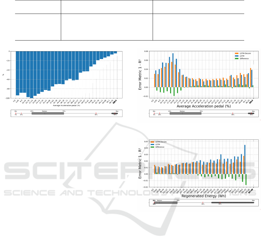
Table 4: Performance metrics comparison for LSTM and LSTM-Decom models across two truck datasets.

Metric LSTM (default) LSTM-Decom (proposed model)

Truck #1 year 2 Truck #2 year 1 Truck #1 year 2 Truck #2 year 1

MAE (Wh) 1229 1397 978 1083

RMSE (Wh) 2122 2340 1722 1880

MAPE (%) 7.4% 8.5% 6.0% 6.6%

Error <10% (%) 74% 66% 82% 79%

Figure 6: Mean regenerative energy across different val-

ues of the average acceleration pedal within segments. The

y-axis is normalized between the minimum and maximum

values for conﬁdentiality reasons. The boxplot beneath the

x-axis indicates the distribution of values within the dataset.

a strong correlation between segments with a low ac-

celeration pedal position and higher amounts of re-

generative energy.

The LSTM-Decom model improves the perfor-

mance speciﬁcally for those segments with a low av-

erage acceleration pedal position, as shown in Fig-

ure 7a. The chosen error metric is one minus the R

scores across segments with different average pedal

position values. The R

is a measure of how much of

the variance in the energy consumptions is explained

by the inputs. As most values are relatively close to 1

the difference to one is used, implying that low values

of this metric indicate good performance.

The improvement in predicting regenerative en-

ergy is conﬁrmed by Figure 7b, where increasingly

higher regenerative energy correlates with higher im-

provements in prediction accuracy for the LSTM-

Decom model. Even with these improvements, the

biggest source of error (derived using the decision

tree method) remains the low average acceleration

pedal position. This might be related to the fact

that the amount of energy that is regenerative is

highly uncertain. Overall, these results show that the

LSTM-Decom model improves prediction accuracy

by leveraging domain knowledge to face the main er-

ror source, leading to a 20% reduction of mean abso-

lute percentage error over both test sets.

(a) 1-R

metric across different values of the average accel-

eration pedal within segments.

(b) 1-R

metric across different values of the average regen-

erative braking within segments.

Figure 7: Energy consumption estimation comparison.

5.3 Uncertainty Scores

The results of the uncertainty-aware models are ﬁrst

evaluated for the prediction interval application by

creating such intervals for conﬁdence terms α = 0.05

and α = 0.01, indicating low and very low tolerance

for errors, respectively. The results in Table 5 provide

the results for both one-sided upper bounds and two-

sided intervals. The former can be used for the de-

sign of worst-case scenarios, whereas the latter gives

a more complete image of the quality of the uncer-

tainty score.

Results show that for 6 out of 8 evaluated

intervals, the LSTM-TMV model produces well-

calibrated scores (see Section 4 for context on the

metrics). For the Gaussian model, this only holds for

3 out of 8 intervals, with several calibration values

VEHITS 2025 - 11th International Conference on Vehicle Technology and Intelligent Transport Systems

174

far from the target (e.g. 75% for the two-sided in-

terval with α = 0.05). When looking at the average

calibration error (distance from 1 − α), the error for

the GMP model is 7.7%, whereas the average calibra-

tion error is only 0.6% for the LSTM-TMV model.

This corresponds to a 92% decrease in calibration er-

ror. As the calibration metric deﬁnes the reliability of

the intervals, the LSTM-TMV model is deemed best

for modeling the uncertainties. However, this comes

at the cost of a higher median sharpness as listed in

Table 5. This means that the intervals for LSTM-

TMV are generally wider than for the GMP model.

When leveraging the score in planning applications,

this results in more “conservative” bounds than the

Gaussian scores.

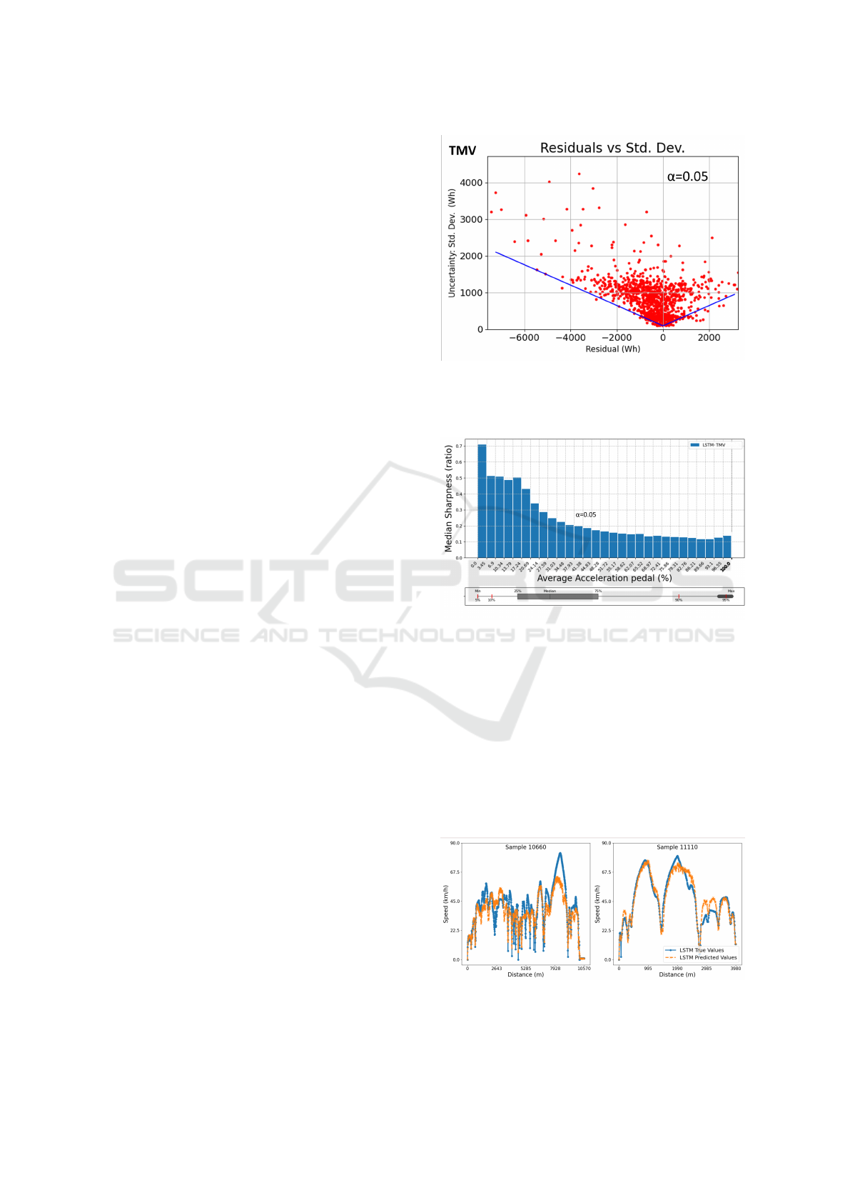
Let us look at another use-case for the uncertainty

score: a decision threshold, below which predictions

are deemed reliable or above which they are marked

as too risky. Figure 8 visualizes the relation be-

tween model error and predicted uncertainty scores.

It shows how a lower bound can be drawn, indicat-

ing that lower uncertainty scores correspond to lower

model errors. Thus, the ﬁgure can aid the end-user in

choosing a suitable threshold. Figure 9 shows that the

median sharpness of generated prediction intervals

using the LSTM-TMV model is higher for lower av-

erage acceleration pedal positions in segments. This

is consistent with what is expected, considering that

many uncertainties are paired with the amount of re-

generative in these cases.

To give an example of the probabilistic use-case

of the uncertainty score, let us evaluate an example

trip selected from the ﬁrst test set. With a predicted

consumption of 20,407 Wh and a predicted standard

deviation of 1069 Wh, a ﬂeet manager might wonder

what the probability is that 22,000 Wh of energy is

enough to complete the trip. Using the CDF function

provided in Section 4.2, a probability of 89.5% is de-

rived.

5.4 Speed Proﬁle Predictor

The results of the LSTM model for speed predictions

are given in Table 6. For the speed prediction and

the full prediction pipeline experiments (Section 5.5)

only the test set for Truck #1 in year 2 is used for

evaluation.

Figure 10 shows the resulting predicted speed pro-

ﬁles for two sampled trips. Generally, the predicted

speed sequences follow the measured speeds, show-

ing the ability to predict acceleration and deceleration

patterns. However, the sample on the left is an exam-

ple of a phenomenon observed throughout the dataset;

the model seems unable to capture high-frequency

Figure 8: Lower bound on the uncertainty score (st.dev) for

all residuals of the LSTM-TMV model on test set “Truck #1

- year 2”. α = 0.05 relates to the design of the lower bound,

such that 95% of the points lie above it.

Figure 9: Visualization of the median sharpness (two-sided

interval with α = 0.05) across different values for the aver-

age acceleration pedal position. The uncertainty scores are

higher for lower acceleration pedal positions.

changes (seen in the middle of the segment) and rather

predicted a smoothed velocity proﬁle. The predicted

speeds around 3000 meters of the sample on the right

show that certain driving behavior was expected (two

peaks) but not measured in the dataset. This shows

how the model can learn patterns, which might de-

pend on uncertainties in driving behavior or the envi-

ronment.

Figure 10: Predicted speed sequences plotted against mea-

sured speed data for two sampled trips in the year 2 for

Truck #1.

Energy Consumption Prediction with Uncertainty Quantiﬁcation for Electric Truck Operations: A Data-Driven Approach

175

Table 5: Quantitative analysis comparing the uncertainty-aware LSTM-GMP and LSTM-TMV models. Calibrations meeting

alpha thresholds are in bold.

Model Comparison LSTM-GMP LSTM-TMV

Dataset Truck #1 Year 2 Truck #2 Year 1 Truck #1 Year 2 Truck #2 Year 1

α = 0.05:

Calibration upper bound 96.44% 97.82% 95.90% 93.67%

Calibration two-sided 75.07% 76.20% 95.37% 95.92%

Median Sharpness 10.22% 10.92% 11.14% 11.86%

Median Sharpness two-sided 24.27% 25.93% 29.01% 30.90%

α = 0.01:

Calibration upper bound 98.13% 99.20% 98.84% 99.53%

Calibration two-sided 91.54% 89.56% 99.11% 99.75%

Median Sharpness 14.40% 15.39% 19.58% 20.85%

Median Sharpness two-sided 31.82% 34.00% 48.11% 51.23%

Table 6: Speed proﬁle results.

Metric Truck #1 Year 2

MAE (km/h) 3.64

RMSE (km/h) 5.59

MdAPE (%) 7%

Table 7: Results on the full prediction pipeline for the

LSTM-Decom and LSTM-TMV models (Trip-level).

Metric LSTM-Decom LSTM-TMV

MAE (Wh) 1507 2253

RMSE (Wh) 2484 3658

MAPE (%) 10.8% 12.50%

Error <10% (%) 59% 40%

5.5 Full Prediction Pipeline

Evaluating the speed proﬁle predictor in combination

with both the LSTM-Decom model as well as the

LSTM-TMV model leads to the results in Table 7.

The LSTM-Decom model shows a mean absolute pre-

diction error of 10.8% and predicts 59% of segments

with an error of 10% or below, showing suitable per-

formance for a majority of segments. Compared to

the evaluations for the energy consumption models in

Section 5.2, higher errors are observed for the full

prediction pipeline. Given the presence of predic-

tion errors for the speed model, this decline in per-

formance is expected. The calibration of the LSTM-

TMV model in the full prediction pipeline as seen in

Table 8 is slightly below the target rate for the pre-

dicted intervals and alpha values. This is most likely

because the uncertainty in the predicted speed is not

accounted for. Still, the calibrations are generally

high, indicating that the scores convey meaningful in-

formation about the underlying uncertainties.

Table 8: Calibration and sharpness results for Truck #1 year

2 at different alpha values.

Metric

Truck #1

Year 2

α = 0.05:

Calibration upper bound 90.45%

Calibration two-sided 77.61%

Median Sharpness 11.63%

Median Sharpness two-sided 30.29%

α = 0.01:

Calibration upper bound 95.72%

Calibration two-sided 94.56%

Median Sharpness 20.44%

Median Sharpness two-sided 50.23%

6 CONCLUSIONS AND FUTURE

WORK

Motivated by the increasing adoption of battery-

electric trucks and their operational challenges related

to energy consumption prediction, this work investi-

gated a two-stage data-driven approach to predict the

energy consumption of electric trucks. The approach

integrated a speed proﬁle predictor and an energy con-

sumption estimator.

The key ﬁndings of this paper improve the energy

consumption estimator or provide a measure of the

uncertainty in the predictions. In the ﬁrst key ﬁnd-

ing, the energy consumption estimation is improved

by including the novel Long Short-Term Memory

(LSTM)-Decom architecture, which decomposes the

energy consumption into regenerative and consumed

energy. The second key ﬁnding produces an uncer-

tainty measure in the energy prediction. Compared

to the state-of-the-art Gaussian uncertainty scores,

VEHITS 2025 - 11th International Conference on Vehicle Technology and Intelligent Transport Systems

176

the implemented LSTM-TMV approach assumes a t-

distributed error, which successfully produced well-

calibrated prediction intervals.

The approach is evaluated using a real data set

recorded in electric trucks. Results show a mean ab-

solute prediction error of 7.4%, when evaluating only

the energy estimation part (i.e., using true speeds).

The reduction of error compared to a standard LSTM

encoder architecture is 20%, where analysis shows

this is due to improvements in independently predict-

ing regenerative energy. Evaluating the uncertainty

quantiﬁcation scores, the novel t-distributed error ap-

proach reduces the calibration error (when compared

to a Gaussian approach) by as much as 92%.

The resulting approach shows a mean absolute

prediction error of 10.8%, when both the speed and

energy consumption are estimated (i.e., the combined

pipeline). The decrease in the prediction error com-

pared to state-of-the-art techniques and the provided

uncertainty in prediction error make the approach

suitable for planning operations.

Future work approaches focus on improving the

pipelined by including probabilitic approaches to pre-

dict speed, exploring unceratainty propagation from

speed to energy prediction, and enhance the data-

driven predictions by levearaging from the insights

provided by the well-know vehicle physic behaviour.

ACKNOWLEDGEMENTS

This work has received ﬁnancial support from the

Dutch Ministry of Economic Affairs and Climate, un-

der the grant ‘R&D Mobility Sectors’, projects Green

Transport Delta - Electriﬁcatie (GTD-e) and Charging

Energy Hubs (CEH), and the European Union’s Hori-

zon 2020 research and innovation programme under

grant agreement No 101192657, under the title of

FlexMCS.

REFERENCES

Basso, R. (2019). Energy consumption estimation in-

tegrated into the Electric Vehicle Routing Problem.

Transportation Research Part D: Transport and En-

vironment, 69:141–167.

Chen, Y. (2021a). Data-driven estimation of energy con-

sumption for electric bus under real-world driving

conditions. Sustainable Transport, Energy, Environ-

ment, & Policy, 98:102969.

Chen, Y. (2021b). A Review and Outlook of Energy Con-

sumption Estimation Models for Electric Vehicles.

SAE International Journal of Sustainable Transporta-

tion, Energy, Environment, & Policy.

De Cauwer, C. (2017). A Data-Driven Method for Energy

Consumption Prediction and Energy-Efﬁcient Rout-

ing of Electric Vehicles in Real-World Conditions. En-

ergies, 10(5):608.

DriveToZero (2024). Memorandum of understanding (mou)

on zero-emission medium- and heavy-duty vehicles.

online.

Dutch Government (2019). National climate agreement.

Policy report on adaptation and mitigation strategies

to combat climate change.

Feng, Z. (2024). Energy consumption prediction strat-

egy for electric vehicle based on LSTM-transformer

framework. Energy, page 131780.

Fiori, C., Ahn, K., and Rakha, H. A. (2016). Power-

based electric vehicle energy consumption model:

Model development and validation. Applied Energy,

168:257–268.

Fotouhi, A. (2021). Electric vehicle energy consumption es-

timation for a ﬂeet management system. International

Journal of Sustainable Transportation, 15(1):40–54.

International Energy Agency (IEA) (2024). Global

EV outlook 2024. https://www.iea.org/reports/

global-ev-outlook-2024. Licence: CC BY 4.0.

Ministry of Infrastructure and Water Management (2024).

Zero-emissiezones in nederland. Web page. Informa-

tion about the implementation dates and locations of

zero-emission zones in 29 Dutch municipalities. Ac-

cessed: 01-07-2024.

Nan, S. (2022). From driving behavior to energy consump-

tion: A novel method to predict the energy consump-

tion of electric bus. Energy, 261:125188.

Pan, Y. (2023). Development of an energy consumption

prediction model for battery electric vehicles in real-

world driving: A combined approach of short-trip seg-

ment division and deep learning. Journal of Cleaner

Production, 400:136742.

Pelletier, S. (2019). The electric vehicle routing problem

with energy consumption uncertainty. Transp. Re-

search Part B, 126:225–255.

Petkevicius, L. (2021). Probabilistic Deep Learning for

Electric-Vehicle Energy-Use Prediction. In 17th

International Symposium on Spatial and Temporal

Databases, pages 85–95, virtual USA. ACM.

Thorgeirsson, A. (2021). Probabilistic Prediction of Energy

Demand and Driving Range for Electric Vehicles With

Federated Learning. IEEE Open Journal of Vehicular

Technology, 2:151–161.

Wu, X. (2015). Electric vehicles’ energy consumption mea-

surement and estimation. Transportation Research

Part D: Transport and Environment, 34:52–67.

Yang, S. (2014). Electric vehicle’s electricity consumption

on a road with different slope. Statistical Mechanics

and its Applications, 402:41–48.

Energy Consumption Prediction with Uncertainty Quantiﬁcation for Electric Truck Operations: A Data-Driven Approach

177