Assessing Human Activity in Elderly People’s Homes Using the
Dempster-Shafer Theory
Sanamjeet Meyer
a
, Sebastian Wilhelm
b
, and Florian Wahl
c
Deggendorf Institute of Technology, Dieter-G
¨
orlitz-Platz 1, 94469 Deggendorf, Germany
Keywords:
Human Activity Recognition, Uncertainty Quantification, Ambient Assisted Living, Activities of Daily Living.
Abstract:
The increasing elderly population living alone, alongside caregiver shortages, has accelerated research in
Ambient Assisted Living (AAL). A recent trend employs smart meters and Non-Intrusive Load Monitoring
(NILM) to assess daily activities by analyzing device-specific power usage. This work explores the use of
Dempster-Shafer Theory (DST) to enhance NILM-based anomaly detection in daily routines. Evaluated on
the SynD dataset, our approach identifies deviations such as unexpected appliance use and inactivity. Results
demonstrate DST’s potential for non-intrusive elderly monitoring, with future research focusing on real-world
validation.
1 INTRODUCTION
By 2050, the population of people aged 65+ is pro-
jected to rise significantly (Eurostat, 2020). Over
the last 20 years, the number of elderly living alone
has increased by 19 %. In Germany, 96 % of those
aged 65+ live in private homes, with only 4 % in
nursing homes (Destatis, 2023). Many prefer inde-
pendent living, yet loneliness and social isolation in-
crease the risk of dementia (Lazzari and Rabottini,
2022). A survey across 10,000 individuals aged 80+
in Germany found that 18.1 % suffered from demen-
tia and 24.9 % had mild cognitive problems (Brijoux
and Zank, 2023). The ageing population and care-
giver shortage, have led to extensive research in Am-
bient Assisted Living (AAL) (Alcala et al., 2017b).
AAL leverages technology and data collection to
support elderly care. Monitoring methods are cat-
egorized into direct (wearable sensors) and indirect
(environmental sensors). While direct methods pro-
vide precise physiological data (e.g. heart rate), they
are intrusive and suited for high-risk patients (Alcala
et al., 2017b). Indirect methods, such as motion sen-
sors, are less accepted due to cost and perceived intru-
siveness (Chalmers et al., 2016; Alcala et al., 2015).
Smart meters, increasingly deployed to modernize
electricity networks (McLoughlin et al., 2015), record
a
https://orcid.org/0009-0005-7289-8264
b
https://orcid.org/0000-0002-4370-9234
c
https://orcid.org/0000-0002-1163-1399
real-time energy consumption and transmit data for
monitoring and billing (Zheng et al., 2013). Their
widespread adoption presents a scalable alternative to
traditional ambient sensors.
Non-Intrusive Load Monitoring (NILM) enables
monitoring of Activities of Daily Living (ADLs) via
household appliance usage (Bousbiat et al., 2022).
Proposed by Katz, ADLs include essential tasks like
eating and bathing (Katz et al., 1963). Deviations
in energy data may indicate early cognitive decline
(Bousbiat et al., 2022). The challenge lies in detect-
ing such deviations reliably.
This paper provides the following contributions:
1. A framework for applying Dempster-Shafer The-
ory (DST) to detect human activity from smart
meter data.
2. A method for inactivity pattern detection.
3. A classification method to identify anomalies in
elderly daily activities.
2 RELATED WORK
Alcala et al. (2017a, 2015, 2017b) have significantly
contributed to NILM-based human activity assess-
ment. Their first approach (Alcala et al., 2015) uti-
lizes a difference Hidden Markov Model (HMM) to
detect appliance use from aggregated smart meter
data and models appliance occurrences via a Poisson
distribution with a log Gaussian Cox process. The
Meyer, S. S., Wilhelm, S. and Wahl, F.
Assessing Human Activity in Elderly People’s Homes Using the Dempster-Shafer Theory.
DOI: 10.5220/0013354100003938
Paper published under CC license (CC BY-NC-ND 4.0)
In Proceedings of the 11th International Conference on Information and Communication Technologies for Ageing Well and e-Health (ICT4AWE 2025), pages 291-301
ISBN: 978-989-758-743-6; ISSN: 2184-4984
Proceedings Copyright © 2025 by SCITEPRESS – Science and Technology Publications, Lda.
291

method, evaluated on the HES dataset, enabled early
intervention in 25 of 35 households and reduced false
alarms. This study extends their work by incorporat-
ing multiple appliances.
Alcala et al. (2017a,b) also compared Gaussian
Mixture Model (GMM) and DST for monitoring
household activity. GMM trains probabilistic ap-
pliance models, computing a daily likelihood score,
while DST generalizes Bayesian theory by defin-
ing belief and plausibility bounds to handle uncer-
tainty in non-deterministic human behavior. Demp-
ster’s rule of combination aggregates belief assign-
ments from different appliances, providing a normal-
ity score. DST outperformed GMM in detecting
short- and long-term deviations (Alcala et al., 2017b).
This study implements DST to simulate behavioral
changes and emergencies.
Bousbiat et al. (2022) propose an interactive
framework for activity monitoring based on user pro-
files, integrating load disaggregation, activity track-
ing, and feedback management. Activities are mod-
eled via activity curves and self-similarity measures,
stored in an observation database. Daily reports
are compared using the Jensen-Shannon Divergence.
While some anomalies were undetected, the frame-
work showed overall acceptable performance, though
it relied on single-appliance analysis.
Chalmers et al. (2019) explored NILM for ADLs
assessment in dementia care. A six-month clinical
trial tested Support Vector Machine and Random De-
cision Forest classifiers, achieving high sensitivity in
detecting appliances. Behavioral patterns were mod-
eled as feature vectors, analyzed through seven ob-
servation windows, Sankey diagrams, and Z-scores to
detect anomalies. The approach successfully iden-
tified behavioral changes such as sundowning syn-
drome. Inspired by this, we evaluate DST for detect-
ing similar conditions.
3 METHODOLOGY
Our approach extends Alcala et al. (2017b) by di-
viding the process into two phases: Observation and
Evaluation. We first introduce DST.
3.1 Dempster-Shafer Theory (DST)
DST generalizes Bayesian probability theory and
provides a framework for handling epistemic un-
certainty (Sentz and Ferson, 2002). Instead of
assigning precise probabilities, it maps probability
mass to sets or intervals, interpreted as evidential
weights (Rakowsky, 2007). DST consists of three
components: basic assignment, belief and plausibil-
ity, and Dempster’s rule of combination.
3.1.1 Basic Assignment
Basic assignment, denoted by m, maps the power set
2
Ω
to the interval [0, 1]:
m : 2
Ω
→ [0, 1] (1a)
m(
/
0) = 0 (1b)
∑
A⊆2
Ω
m(A) = 1 (1c)
Unlike probability functions, m does not necessar-
ily satisfy m(Ω) = 1, nor does m(A) ≤ m(B) if A ⊂
B (Rakowsky, 2007).
3.1.2 Belief and Plausibility
Belief bel(A) sums basic assignments for subsets B ⊆
A, while plausibility pl(A) sums assignments for sets
where B ∩ A ̸=
/
0:
bel(A) =
∑
B⊆A;B̸=
/
0
m(B) (2a)
pl(A) =
∑
B∩A̸=
/
0
m(B) (2b)
bel(a) ≤ m(A) ≤ pl(a) (2c)
The difference pl(A) − bel(A) quantifies uncer-
tainty (Klir and Wierman, 1999). Belief and plausi-
bility should not be seen as complementary but rather
as bounds on probability.
3.1.3 Dempster’s Rule of Combination
Dempster’s rule aggregates independent basic assign-
ments m
1
and m
2
:
m
1,2
(
/
0) = 0 (3a)
m
1,2
(A) =
∑
B∩C=A̸=
/
0
m
1
(B)m
2
(C)
1 − K
(3b)
K =
∑
B∩C=
/
0
m
1
(B)m
2
(C) (3c)
The denominator normalizes conflicting assign-
ments (Shafer, 1986).
3.2 Applying DST to Asses Human
Activity
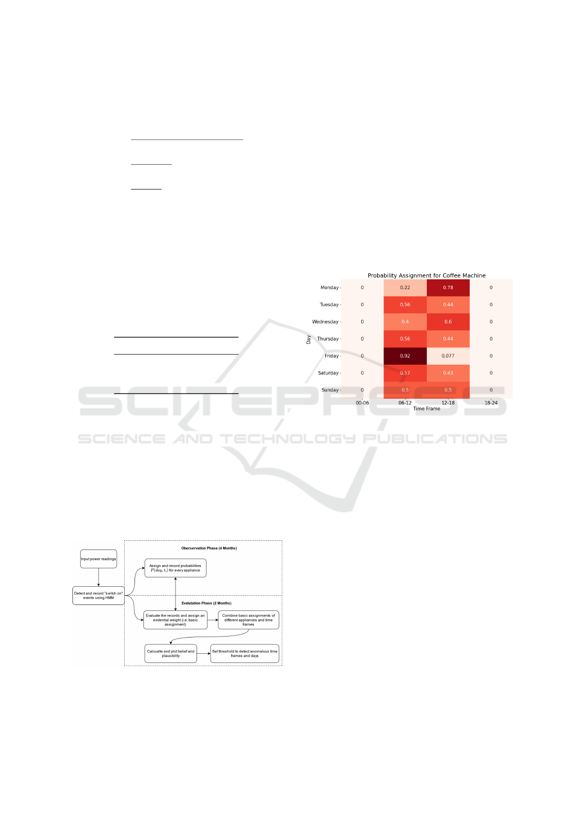
3.2.1 Observation Phase
Household activities are recorded over four months
using individual appliance power readings from the
SynD dataset (Klemenjak et al., 2020) and a HMM to
detect ’switch-on’ events.
ICT4AWE 2025 - 11th International Conference on Information and Communication Technologies for Ageing Well and e-Health
292

3.2.2 Recording Activities and Probability
Assignment
Whenever a ’switch on’ event is detected, the times-
tamp is recorded and assigned to one of four time bins
(t
i
) of six-hour intervals. This process is repeated for
each date and all appliances under consideration.
After the observation phase, the data is stored in a
Pandas data frame. The value at index (day,t
i
) repre-
sents the frequency of appliance use for a given day
and time frame. Probabilities P(t
i
) are then assigned
by normalizing each row (n) by its total count (N):
P(day,t
i
) = n
day,t
i
/N
day
(4)
3.2.3 Evaluation Phase
After the observation phase and probability assign-
ment, DST is applied to assess household activi-
ties. This involves computing basic assignments (Sec-
tion 3.2.4), combining them across appliances and
time frames (Section 3.2.5), and deriving belief and
plausibility measures.
The frame of discernment (Ω) consists of two hy-
potheses: ’normal pattern’ (h
1
) and ’abnormal pat-
tern’ (h
2
). The power set (2
Ω
) also includes the com-
bined hypothesis ’normal or abnormal pattern’ (h
3
)
and the null set (
/
0):
h
1
(normal pattern), h
2
(abnormal pattern) (5a)
h
3
= h
1
∪ h
2
(normal or abnormal pattern) (5b)
Ω = {h
1
,h
2
}, 2
Ω
= {
/
0,h
1
,h
2
,h
3
} (5c)
3.2.4 Basic Assignment and Weighing
Basic assignments are computed based on detected
’switch-on’ events. When the HMM detects a tran-
sition from ’off’ to ’on’, the timestamp is stored in
a Pandas data frame. For each time frame t
i
, the
recorded event count is used to weigh probabilities
P(day,t
i
), as defined in Equations 6.
m
date,t
i
(h
1
) =
(
P(day,t
i
) ×C
0
, if event
(1 − P(day,t
i
)) ×C
1
, if not event
(6a)
m
date,t
i
(h
2
) =
(
(1 − P(day,t
i
)) ×C
0
, if event
P(day,t
i
) ×C
1
, if not event
with ∆t
i
∈ [0, 24) (6b)
m
date,t
i
(h
3
) = 1 −(m
date,t
i
(h
1
) + m
date,t
i
(h
2
)) (6c)
The certainty constants C
0
and C
1
(ranging from 0
to 1) encode uncertainty and depend on appliance us-
age. In Alcala et al. (2017b), they were empirically
set to C
0
= 0.9 and C
1
= 0.1, with a 6-hour evaluation
window. This implies a 10 % uncertainty in event de-
tection and 90 % in event absence.
Absence of an event does not necessarily indi-
cate an abnormal pattern, as human behavior is unpre-
dictable. DST manages uncertainty, unlike Bayesian
approaches that rely solely on probabilities. Further-
more, event occurrence does not inherently imply nor-
mality but contributes additional information, reduc-
ing uncertainty by 10 % (Alcala et al., 2017b).
3.2.5 Combining Basic Assignments
After computing basic assignments (Section 3.2.4),
Dempster’s rule of combination aggregates them
across appliances and time frames t
i
. This ensures
that evidence from multiple sources contributes to an
overall activity assessment.
To illustrate the process, Table 1 presents arbitrary
basic assignments for appliances X and Y .
Table 1: Basic assignments for appliances X and Y (Alcala
et al., 2017b).
Appliance X 2
Ω
Appliance Y
m
date,t
i
(h
1
) = 0.8 h
1
m
date,t
i
(h
1
) = 0.6
m
date,t
i
(h
2
) = 0.1 h
2
m
date,t
i
(h
2
) = 0.2
m
date,t
i
(h
3
) = 0.1 h
1
∪ h
2
m
date,t
i
(h
3
) = 0.2
Each set of hypotheses is then combined by com-
puting intersections, as shown in Table 2. The inter-
section of h
1
and h
2
is the empty set, as both patterns
cannot coexist.
Table 2: Combining sets of hypotheses for appliances X and
Y (Alcala et al., 2017b).
∩ h
1
x
h
2
x
h
3
x
h
1
y
h
1
/
0 h
1
h
2
y
/
0 h
2
h
2
h
3
y
h
1
h
2
h
3
Table 3 represents the product of basic assign-
ments for appliances X and Y .
Table 3: Products of basic assignments for appliances X and
Y (Alcala et al., 2017b).
· m(h
1
)
x
m(h
2
)
x
m(h
3
)
x
m(h
1
)
y
0.6 · 0.8 0.6 · 0.1 0.6 · 0.1
m(h
2
)
y
0.2 · 0.8 0.2 · 0.1 0.2 · 0.1
m(h
3
)
y
0.2 · 0.8 0.2 · 0.1 0.2 · 0.1
The combined basic assignments (m(h
1
), m(h
2
),
Assessing Human Activity in Elderly People’s Homes Using the Dempster-Shafer Theory
293

m(h
3
)) are calculated using:
K = 0.8 · 0.2 + 0.6 · 0.1 (7a)
m(h
1
) =
0.8 · 0.6 +0.1 · 0.6 + 0.8 · 0.2
1 − K
(7b)
m(h
2
) =
0.1 · 0.2 ·3
1 − K
(7c)
m(h
3
) =
0.1 · 0.2
1 − K
(7d)
Finally, belief and plausibility measures are com-
puted as follows:
bel(h
1
) = 0.89, pl(h
1
) = 0.92 (8a)
bel(h
2
) = 0.08, pl(h
2
) = 0.1 (8b)
bel(h
3
) = 1, pl(h
3
) = 1 (8c)
Table 4 summarizes the results.
Table 4: Summary of results (Alcala et al., 2017b).
2
Ω
m(t
i
) bel(t
i
) pl(t
i
)
h
1
0.89 0.89 0.92
h
2
0.08 0.08 0.1
h
3
0.02 1 1
The same process is repeated across time frames
to accumulate a daily basic assignment.
4 EVALUATION
4.1 Overview
Figure 1 presents the workflow, from data ingestion
and power processing to the identification of anoma-
lies based on belief and plausibility thresholds.
Figure 1: Workflow overview.
Selected appliances should be frequently used,
manually operated, and associated with ADLs. We
chose an electric kettle, coffee machine, microwave,
television, hairdryer, toaster, and mini oven. Their
high power consumption enhances detectability in
NILM-based disaggregation. Unlike Alcala et al.
(2017b), we excluded low-power appliances such as
lamps.
4.2 Observation Phase Workflow
Power readings from the selected appliances were
split into observation (4 months) and evaluation
(2 months) data. ’Switch-on’ events detected by
the HMM were recorded for probability assign-
ment 3.2.2. Figure 2 visualizes probability distribu-
tions for the coffee machine.
Figure 2: Probability assignment for coffee machine.
4.3 Evaluation Phase Workflow
The last two months of data were used for evaluation.
Detected ’switch-on’ events were mapped to proba-
bility assignments (P(day,t
i
)), and basic assignments
were accumulated across appliances and time frames
to create a daily activity profile.
5 RESULTS
This Section discusses the results obtained using the
workflow shown in Figure 1, focusing on the eval-
uation phase. It also covers how this DST con-
figuration handles simulated emergencies and be-
havioural changes resulting from manipulating inter-
mediate steps.
5.1 Plotting Belief and Plausibility
Once the evaluation phase begins and the basic as-
signments are mapped, the belief and plausibility
measures are calculated and plotted on a line chart as
ICT4AWE 2025 - 11th International Conference on Information and Communication Technologies for Ageing Well and e-Health
294

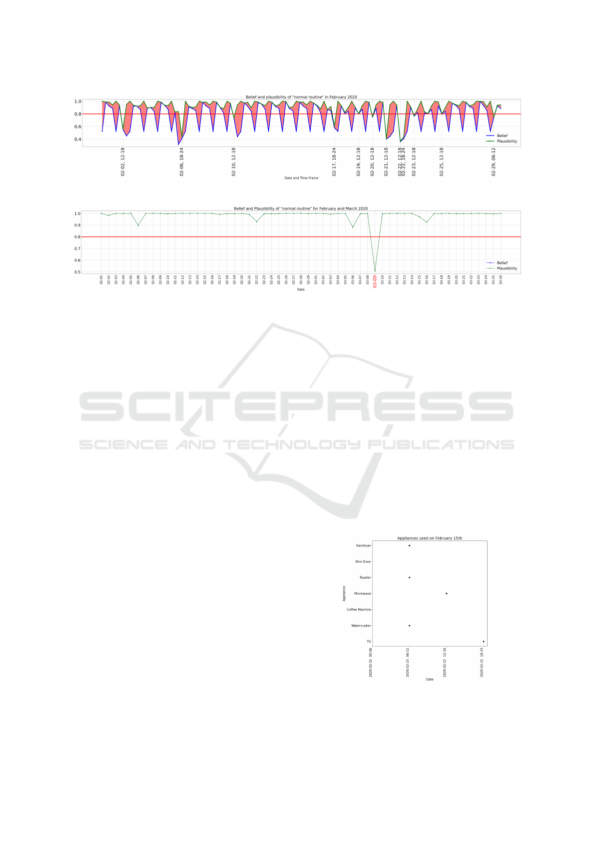
Figure 3: Belief and plausibility of h
1
in February 2020 (accumulated basic assignment of appliances).
Figure 4: Belief and plausibility of h
1
(accumulated basic assignment of appliances and time frames).
suggested by Alcala et al. (2017b). Figures 3 and 7a
display the belief and plausibility of the accumulated
basic assignments of various appliances for February
and March 2020, represented by the blue and green
line respectively. The size of the red area between
these lines indicates the level of uncertainty. There-
fore, the larger the red area, the more uncertainty there
is regarding h
1
(’normal pattern’). Accumulating for
a daily basic assignment reduces the uncertainty, as
shown in Figure 4. As it is done in the original study
(Alcala et al., 2017b) a line at y = 0.8 represents the
threshold. Therefore, if the value of plausibility and
belief for a given time frame or day are below 0.8,
it is considered ’anomalous’. Dates and time frames
considered ’anomalous’ are displayed on the x-axis.
5.2 Chart Analysis
Monday, March 9th, is the only day on the daily basic
assignment chart in Figure 4 that is below the thresh-
old. The appliances used on this day and the time
frame in which they were used are shown in Table 5.
Any differences between the expected and actual use
of appliances in regards to the time frame, as well as
the resulting increase in belief assignment for the cor-
responding hypothesis, are also shown in Table 5.
Unexpected appliance usage increases the belief
assignment (m) in both the expected and actual usage
time frames. Consequently, basic assignments m(h
2
)
and m(h
3
) rise, as shown in columns 4 and 5 of Ta-
ble 5. This indicates that unexpected usage raises
m(h
2
), while absence increases m(h
3
).
6 SIMULATING ANOMALOUS
BEHAVIOUR
The appliance usage data showed no signs of anoma-
lous behaviour. Therefore, we tried to simulate
anomalous behaviour, taking into consideration the
baseline usage patterns of the appliances considered.
This is done by changing intermediate steps. Because
of how DST works, it’s easy to simulate emergencies.
All that needs to be done is to add events at odd times
or remove events within a certain time frame. To add
or remove an event, the number of detected ’switch-
on’ events in a given time frame can be either set to 0
or 1. From now on, February 15th will be used to test
different situations. Appliances used on this day are
shown in Figure 5, and the accumulated basic assign-
ments of appliances are presented in Table 6a.
Figure 5: Appliances used on February 15th, 2020.
Assessing Human Activity in Elderly People’s Homes Using the Dempster-Shafer Theory
295

Table 5: Appliances used on March 9th and the subsequent increase basic assignment m.
Appliance Expected Use Actual Use
Increase
(Expected t
i
)
Increase
(Actual t
i
)
Coffee Machine 12-18 06-12 h
3
h
2
Toaster 06-12 - - h
3
Electric Oven 06-12 12-18 h
3
h
2
Television 18-24 12-18 h
3
h
2
Table 6: Comparison of basic assignments on February 15th.
(a) Basic assignments on February 15th (not manipulated).
t
i
m(h
1
) m(h
2
) m(h
3
)
00-06 0.5217 0.0 0.4783
06-12 0.9822 0.0164 0.0014
12-18 0.9222 0.0143 0.0635
18-24 0.8849 0.0592 0.0559
15.02 0.99 0.0 0.0
(b) Basic assignments on February 15th (midday inactivity).
t
i
m(h
1
) m(h
2
) m(h
3
)
00-06 0.5217 0.0 0.4783
06-12 0.9822 0.0164 0.0014
12-18 0.2884 0.1888 0.5228
18-24 0.8849 0.0592 0.0559
15.02 0.99 0.0 0.0
(c) Basic assignments on February 15th (half day inactivity).
t
i
m(h
1
) m(h
2
) m(h
3
)
00-06 0.5217 0.0 0.4783
06-12 0.9822 0.0164 0.0014
12-18 0.2884 0.1888 0.5228
18-24 0.4522 0.0489 0.4989
15.02 0.996 0.0041 0.0002
(d) Basic assignments on February 15th (unusual activity).
t
i
m(h
1
) m(h
2
) m(h
3
)
00-06 0.0810 0.8271 0.0919
06-12 0.9822 0.0164 0.0014
12-18 0.9222 0.0143 0.0635
18-24 0.8849 0.0592 0.0559
15.02 0.99 0.0 0.0
6.1 Midday Inactivity
To simulate midday inactivity, microwave use is re-
moved in the 12-18 time frame. This change increases
the uncertainty for this period. Consequently, the ba-
sic assignment m(h
3
) increases and m(h
1
) decreases
as shown in Tables 6a and 6b.
6.2 Half-Day Inactivity
Half-day inactivity builds on midday inactivity by re-
moving television use after 18:00hrs. As with the re-
moval of microwave use in midday inactivity, the re-
moval of television use also increases uncertainty in
the 18-24 time frame as shown in Tables 6a and 6c.
6.3 Activity at an Unusual Time
Adding events to unusual time frames is a method of
simulating abnormal activity. Between the hours of
00-06 and 18-24, there is typically less activity than
during the other hours. Therefore, the use of a coffee
machine during the time frame 00-06 has been added.
Compared to the half-day and midday inactivity, this
leads to a decrease in uncertainty and increases the
basic assignment m(h
2
) instead of m(h
3
) as shown in
Table 6d. As it was the case for the previous simula-
tions, there is no effect on the daily basic assignment.
7 SIMULATING BEHAVIOURAL
CHANGES
Deviations from regular daily routines, accompanied
by changes in behaviour, may indicate the presence of
dementia. These abnormalities tend to become more
frequent and severe as dementia progresses (Chalmers
et al., 2019). In this section, the results of simulat-
ing sundowning syndrome and mild cognitive impair-
ment, which is a precursor to dementia, are presented.
7.1 Sundowning Syndrome
One well-known condition in dementia patients is the
sundowning syndrome, where a person may exhibit
certain behaviours in the latter half of the day. Moni-
toring power consumption over time can help identify
these behavioural changes (Chalmers et al., 2019).
ICT4AWE 2025 - 11th International Conference on Information and Communication Technologies for Ageing Well and e-Health
296

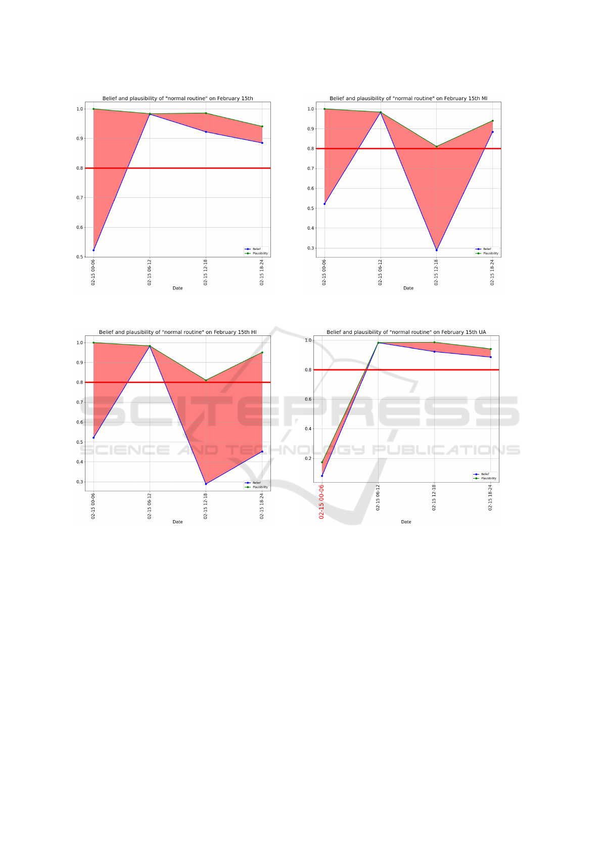
(a) Belief and plausibility on February 15th (not manipu-
lated).
(b) Belief and plausibility on February 15th (midday inactiv-
ity).
(c) Belief and plausibility on February 15th (half day inactiv-
ity).
(d) Belief and plausibility on February 15th (unusual activ-
ity).
Figure 6: Comparison of belief and plausibility on February 15th.
To simulate this, random events were added in the
March 12-18 and 18-24 time frames, including ran-
dom use of the kettle, coffee machine and toaster. Fig-
ures 7b and 8a illustrate the effect of these randomly
added events. Compared to the original results, where
only 16 time frames were considered anomalous, 32
time frames are now considered abnormal. Similarly,
the impact is evident in the daily accumulated ba-
sic assignments chart, which now shows 8 abnormal
days compared to only one previously. In total, all 16
time frames that were previously considered normal
now have time frames with at least one random event
added to them.
7.2 Mild Cognitive Impairment
Memory is one of the first skills of daily living to
be impaired in people with mild cognitive impair-
ment (Scheerbaum et al., 2023). To simulate this,
the events of the same appliances were randomly re-
moved from the time frames 06-12 and 12-18. (see
Figures 7c and 8b) As evident in Figure 7c, there are
visibly more time frames now considered anomalous.
Prior to the events being removed, 16 time frames
were considered anmoulous. Now the number of time
frames considerd anmoulous is 21. Only in about half
of the cases where events were removed from certain
Assessing Human Activity in Elderly People’s Homes Using the Dempster-Shafer Theory
297

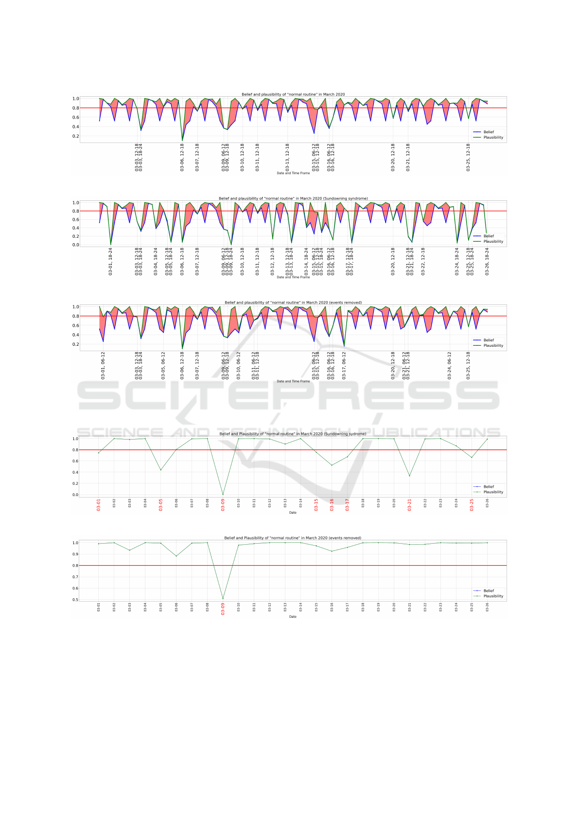
(a) Belief and plausibility of h
1
in March 2020.
(b) Belief and plausibility of h
1
in March 2020 (Sundowning syndrome).
(c) Belief and plausibility of h
1
in March 2020 (Mild cognitive impairment).
Figure 7: Effect of randomly removed events.
(a) Belief and plausibility of h
1
March 2020 (Sundowning syndrome).
(b) Belief and plausibility of h
1
March 2020 (Mild cognitive impairment).
Figure 8: Effect of randomly added events.
time frames did this affect their ’normality’. These
figures should not be interpreted as a measure of ac-
curacy. Figure 8b, which is the plot for the daily ba-
sic assignments for March 2020, still shows the 9th
March 2020 as the only anomalous day.
ICT4AWE 2025 - 11th International Conference on Information and Communication Technologies for Ageing Well and e-Health
298

Table 7: Appliance used on March 9th and the subsequent increase in basic assignment (reconfigured).
Appliance Expected Use Actual Use
Increase
(Expected t
i
)
Increase
(Expected t
i
)
Coffee Machine 12-18 06-12 h
2
h
3
Toaster 06-12 - - h
2
Electric Oven 06-12 12-18 h
2
h
3
Television 18-24 12-18 h
2
h
3
8 DISCUSSION
8.1 Analyzing Dempster’s Rule of
Combination
Analyzing the results in Section 5 reveals key obser-
vations. Unexpected appliance use increases m(h
2
)
in the actual usage time frame and m(h
3
) in the ex-
pected one. Conversely, if an appliance is not used
when expected, m(h
3
) increases in the respective time
frame. Unusual appliance usage significantly impacts
the accumulated daily basic assignment, affecting be-
lief and plausibility, while inactivity has little effect.
These effects arise because Dempster’s rule dis-
regards h
3
when combining hypotheses, as shown in
Equations 9.
h
1
∩ h
3
= h
1
(9a)
h
2
∩ h
3
= h
2
(9b)
As a result, missing events do not affect daily ba-
sic assignments. This explains why a single omitted
event had little impact, as seen in Section 7.2.
8.2 Evaluating the Basic Assignment
Configuration
As shown in Equations 10, a high evidential weight is
assigned to h
3
even when the probability of use is low.
This results from the certainty constants (C
0
= 0.9,
C
1
= 0.1), which attribute high uncertainty to inactiv-
ity. The original study (Alcala et al., 2017b) included
appliances like lamps and printers, which are rarely
used or have low power consumption. Assigning high
uncertainty ensures these cases are disregarded (Sec-
tion 8.1).
Inactivity
High Probability
P(t
i
) = 0.8 (10a)
m(h
1
) = (1 − 0.8) × 0.1 = 0.02 (10b)
m(h
2
) = 0.8 × 0.1 = 0.08 (10c)
m(h
3
) = 1 − (0.02 + 0.08) = 0.9 (10d)
Low Probability
P(t
i
) = 0.2 (10e)
m(h
1
) = (1 − 0.2) × 0.1 = 0.08 (10f)
m(h
2
) = 0.2 × 0.1 = 0.02 (10g)
m(h
3
) = 1 − (0.02 + 0.08) = 0.9 (10h)
Activity
Low Probability
P(t
i
) = 0.2 (10i)
m(h
1
) = 0.2 × 0.9 = 0.18 (10j)
m(h
2
) = (1 − 0.2) × 0.9 = 0.71 (10k)
m(h
3
) = 1 − (0.18 + 0.71) = 0.11 (10l)
8.3 Re-Configuring the Basic
Assignment Process
The basic assignment process is subjective, allowing
it to be reconfigured. Unlike the basic assignment
configuration used by the authors in (Alcala et al.,
2017b), where h
3
is assigned a high evidential weight
on inactivity. In the case of inactivity, this configu-
ration assigns h
2
a high evidential weight. The cer-
tainty constants C
0
and C
1
can be reconfigured to en-
able this. To do this, C
1
can be set to a higher value,
e.g. 0.5, which in turn only assigns a 50 % uncertainty
when an appliance is not used. What makes this fea-
sible is the choice of appliances used for this eval-
uation, as they are more critical to the daily routine
compared to those used for the evaluation in (Alcala
et al., 2017b). Equations 11 show the results of this
configuration. While this configuration initially ap-
pears superior, it presents several issues. First, it does
not account for routine variations. Human behavior
is unpredictable, and earlier or later appliance usage
Assessing Human Activity in Elderly People’s Homes Using the Dempster-Shafer Theory
299

does not necessarily indicate an abnormal pattern. As
a result, March 9th is still classified as anomalous de-
spite only minor deviations in usage times.
Additionally, assigning a high evidential weight to
h
2
during inactivity introduces distortions. If an appli-
ance is used earlier or later than usual, m(h
2
) unneces-
sarily increases in the expected time frame. In periods
of low activity, the absence of expected events inflates
m(h
1
), overshadowing deviations such as missed TV
usage in the 18-24 time frame.
Inactivity
High Probability
P(t
i
) = 0.8 (11a)
m(h
1
) = (1 − 0.8) × 0.7 = 0.14 (11b)
m(h
2
) = 0.8 × 0.7 = 0.56 (11c)
m(h
3
) = 1 − (0.14 + 0.56) = 0.3 (11d)
Low Probability
P(t
i
) = 0.2 (11e)
m(h
1
) = (1 − 0.2) × 0.7 = 0.56 (11f)
m(h
2
) = 0.2 × 0.7 = 0.14 (11g)
m(h
3
) = 1 − (0.14 + 0.56) = 0.3 (11h)
Activity
Low Probability
P(t
i
) = 0.2 (11i)
m(h
1
) = 0.2 × 0.9 = 0.18 (11j)
m(h
2
) = (1 − 0.2) × 0.9 = 0.71 (11k)
m(h
3
) = 1 − (0.18 + 0.71) = 0.11 (11l)
Table 7 illustrates these changes for March 9th.
Despite reconfiguration, the day is still not identified
as anomalous, except for deviations in the 18-24 time
frame, which this approach does not adequately ad-
dress.
8.4 Subjectivity of Anomalies
Defining abnormal activity patterns in the context of
ADL can be challenging due to the non-deterministic
and changeable nature of human behaviour. There-
fore, it is important to distinguish between variation
and deviation. Variations may refer to new habits
and routines adopted by the person. Conversely, de-
viations, are categorical changes in routine that re-
sult in potentially abnormal patterns (Bousbiat et al.,
2022). Bousbiat et al. (2022) ’This can be illustrated
by the following scenario. A change in breakfast time
for several consecutive days is considered a variation.
However, the sudden cancellation of breakfast is con-
sidered a deviation. In summary, both variation and
deviation can be associated with some kind of physi-
cal or cognitive impairment. Therefore, in both cases,
a personal assessment by a professional is necessary.’
9 CONCLUSION AND FUTURE
WORK
Our approach demonstrates potential for assessing
human activity in the elderly. Simulating emergen-
cies and behavioral changes, such as sundowning syn-
drome, yielded promising results. Event additions
were reflected in both time-based and daily activity
charts. However, our method struggles with event
omissions, such as simulating mild cognitive impair-
ment. The increased evidential weight for m(h
3
) in
missing events is disregarded during basic assignment
accumulation as explaned in Section 8.1. Conse-
quently, unless all activity ceases, single-event omis-
sions do not affect the aggregated basic assignment.
For low-performing NILM algorithms, this ro-
bustness prevents missed detections from distorting
results. However, in high-accuracy NILM, unnoticed
inactivity could be problematic. Detecting missed
events is crucial for elderly activity assessment, ne-
cessitating validation on datasets from individuals
with cognitive or physical impairments.
Identifying anomalies, especially inactivity, re-
mains challenging. Plotting belief and plausibility of
h
1
may not be optimal for practical applications. An
automated classification method (Figure 9) could im-
prove anomaly detection. The empirically set thresh-
olds may require statistical optimization for robust-
ness.
Figure 9: Proposal for automated activity classification.
Future research should explore anomaly classi-
fication by tracking appliance-specific basic assign-
ments. Variations in h
1
may provide insights into the
ICT4AWE 2025 - 11th International Conference on Information and Communication Technologies for Ageing Well and e-Health
300

nature of deviations.
ACKNOWLEDGEMENTS
This research was funded by the Hightech Agenda
Bavaria.
REFERENCES
Alcala, J., Urena, J., Hernandez, A., and Gualda, D.
(2017a). Sustainable homecare monitoring system by
sensing electricity data. IEEE Sensors Journal, PP:1–
1.
Alcala, J. M., Parson, O., and Rogers, A. (2015). Detecting
anomalies in activities of daily living of elderly res-
idents via energy disaggregation and cox processes.
Proceedings of the 2nd ACM International Confer-
ence on Embedded Systems for Energy-Efficient Built
Environments.
Alcala, J. M., Urena, J., Hern
´
andez, A., and Gualda, D.
(2017b). Assessing human activity in elderly people
using non-intrusive load monitoring. Sensors, 17(2).
Bousbiat, H., Leitner, G., and Elmenreich, W. (2022). Age-
ing safely in the digital era: A new unobtrusive activ-
ity monitoring framework leveraging on daily interac-
tions with hand-operated appliances. Sensors, 22(4).
Brijoux, T. and Zank, S. (2023). Auswirkungen kogni-
tiver Einschr
¨
ankungen (Demenz) auf Lebensqualit
¨
at
und Versorgung, pages 173–195. Springer Berlin Hei-
delberg, Berlin, Heidelberg.
Chalmers, C., Fergus, P., Monta
˜
nez, C. A. C., Sikdar, S.,
Ball, F., and Kendall, B. (2019). Detecting activities
of daily living and routine behaviours in dementia pa-
tients living alone using smart meter load disaggrega-
tion. IEEE Transactions on Emerging Topics in Com-
puting, 10:157–169.
Chalmers, C., Hurst, W., Mackay, M., and Fergus, P. (2016).
Smart monitoring: An intelligent system to facilitate
health care across an ageing population.
Destatis (2023). Nearly 6 million older people live
alone. https://www.destatis.de/EN/Press/2021/09/
PE21 N057 12411.html. Abrufdatum: 11. November
2023.
Eurostat (2020). Ageing Europe - looking at the lives
of older people in the EU — ec.europa.eu.
https://ec.europa.eu/eurostat/statistics-explained/
index.php?title=Ageing Europe - looking at the
lives of older people in the EU. [Accessed 23-12-
2023].
Katz, S., Ford, A. B., Moskowitz, R. W., Jackson, B. A., and
Jaffe, M. W. (1963). Studies of illness in the aged: the
index of adl: a standardized measure of biological and
psychosocial function. jama, 185(12):914–919.
Klemenjak, C., Kovatsch, C., Herold, M., and Elmenre-
ich, W. (2020). A synthetic energy dataset for non-
intrusive load monitoring in households. Scientific
Data, 7(1).
Klir, G. and Wierman, M. (1999). Uncertainty-based infor-
mation: elements of generalized information theory,
volume 15. Springer Science & Business Media.
Lazzari, C. and Rabottini, M. (2022). Covid-19, loneliness,
social isolation and risk of dementia in older people:
a systematic review and meta-analysis of the relevant
literature. International Journal of Psychiatry in Clin-
ical Practice, 26(2):196–207.
McLoughlin, F., Duffy, A., and Conlon, M. (2015). A
clustering approach to domestic electricity load pro-
file characterisation using smart metering data. Ap-
plied Energy, 141:190–199.
Rakowsky, U. (2007). Fundamentals of the dempster-shafer
theory and its applications to reliability modeling. In-
ternational Journal of Reliability, Quality and Safety
Engineering - IJRQSE, 14.
Scheerbaum, P., Graessel, E., Boesl, S., Hanslian, E.,
Kessler, C. S., and Scheuermann, J.-S. (2023). Are
protective activities and limitations in practical skills
of daily living associated with the cognitive perfor-
mance of people with mild cognitive impairment?
baseline results from the brainfit-nutrition study. Nu-
trients, 15(16).
Sentz, K. and Ferson, S. (2002). Combination of evidence
in dempster-shafer theory.
Shafer, G. (1986). Probability judgment in artificial intelli-
gence. In Machine intelligence and pattern recogni-
tion, volume 4, pages 127–135. Elsevier.
Zheng, J., Gao, D. W., and Lin, L. (2013). Smart meters
in smart grid: An overview. In 2013 IEEE green tech-
nologies conference (GreenTech), pages 57–64. IEEE.
Assessing Human Activity in Elderly People’s Homes Using the Dempster-Shafer Theory
301