MCPro: A Procedural Method for Topologically Correct Isosurface

Extraction Based on Marching Cubes

Julian Stahl

and Roberto Grosso

Visual Computing Erlangen, Friedrich-Alexander-Universit

at Erlangen-N

urnberg, Germany

Keywords:

Isosurface Extraction, Marching Cubes, Topological Correctness, Saddle Points, Trilinear Interpolation.

Abstract:

In this work, we present an innovative procedural algorithm designed for extracting isosurfaces from scalar

data within hexahedral grids. The geometry and the topological features of the intersection of a level set of the

trilinear interpolant with the faces and the interior of a reference unit cell are analyzed. Ambiguities are solved

without the help of lookup tables, generating a topologically correct triangulation of the level set within the cell

that is consistent across cell boundaries. The algorithm is based on constructing and triangulating a polygonal

halfedge data structure that includes contours and critical points of the trilinear interpolant. Our algorithm

is capable of handling many singular cases that were not solved by previous methods. The efﬁcacy and

correctness of the algorithm were tested on a variety of academic and praxis-relevant CT and MRI datasets.

1 INTRODUCTION

Isosurfacing is a technique for visualizing scalar vol-

ume data by extracting a surface with a constant iso-

value. The surface is often represented as a trian-

gle mesh that can be used for further processing and

computations. Marching Cubes (MC) (Lorensen and

Cline, 1987) is the most common isosurfacing algo-

rithm because of its simplicity and performance. It

computes a triangulation of the surface within dis-

cretized cells of the volume based on trilinear inter-

polation between data points. Especially for compu-

tations and mesh processing algorithms, the topology

of the extracted mesh is essential. An isosurfacing

algorithm that guarantees that the generated meshes

are watertight is called topologically consistent. How-

ever, a topologically consistent triangulation does not

necessarily have the same topology as the trilinear

isosurface. If the extracted mesh is homeomorphic

to the trilinear interpolant, it is called topologically

correct. The original version of Marching Cubes is

neither topologically consistent nor correct.

Many improvements have been proposed to make

Marching Cubes topologically correct, but some spe-

cial cases have been often overlooked. March-

ing Cubes uses predeﬁned triangulations stored in a

lookup table and chooses based on 256 cases deter-

mined only by the scalar ﬁeld value on the cell ver-

https://orcid.org/0009-0005-7564-9984

https://orcid.org/0000-0001-5965-5325

tices. However, when considering the trilinear inter-

polant, there is more than one possible triangulation

in some cases. These cases are called ambiguous,

and many different disambiguation techniques have

been proposed. For example, the asymptotic decider

(Nielson and Hamann, 1991) will choose the correct

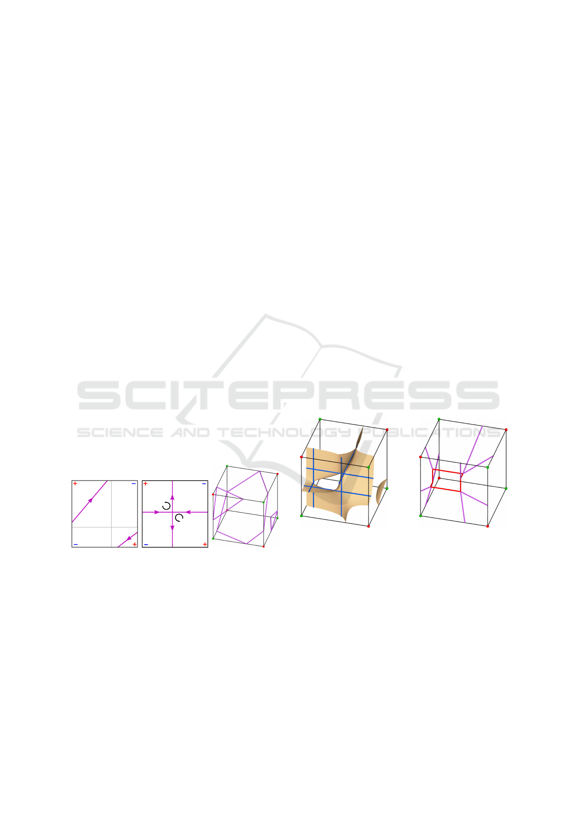
branches of the isosurface. The intersection of an

isosurface of the trilinear interpolant with an axis-

aligned plane is a rectangular hyperbola. The rectan-

gular hyperbola can degenerate into a singular cross,

two axis-aligned lines intersecting at a singular vertex

for a particular combination of the scalar ﬁeld values

as shown in Figure 1.

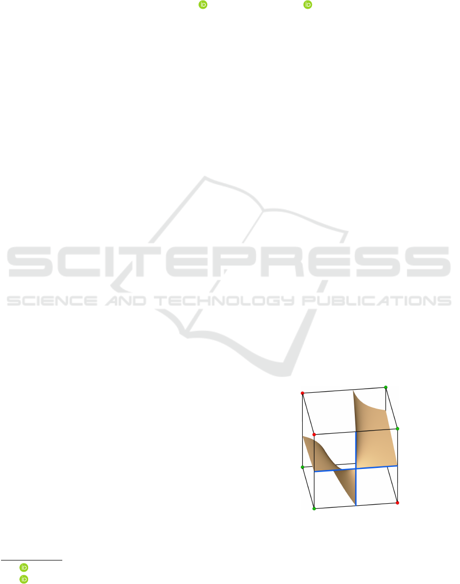
Figure 1: A singular face with a singular point at the inter-

section of the two axis-aligned lines in blue. Positive and

negative corners are marked in green and red.

As we discuss in Section 4, this happens more

frequently in medical data where the resolution of

Stahl, J. and Grosso, R.

MCPro: A Procedural Method for Topologically Correct Isosurface Extraction Based on Marching Cubes.

DOI: 10.5220/0013309800003912

Paper published under CC license (CC BY-NC-ND 4.0)

In Proceedings of the 20th Inter national Joint Conference on Computer Vision, Imaging and Computer Graphics Theory and Applications (VISIGRAPP 2025) - Volume 1: GRAPP, HUCAPP

and IVAPP, pages 331-338

ISBN: 978-989-758-728-3; ISSN: 2184-4321

331

values is often limited to integers. In such cases,

the disambiguation approaches fail to determine

the correct topology of the isosurface. Therefore,

we propose a new isosurfacing algorithm based on

Marching Cubes that generates topologically correct

triangulations and can handle singular cases that

other methods cannot solve. The triangulations are

computed procedurally without using a lookup table,

which avoids hand-crafting and storing a large num-

ber of possible conﬁgurations. The algorithm utilizes

simple properties of the isosurface and the trilinear

interpolation for robust topology disambiguation.

The contributions of this paper are:

• a lookup table-free, procedural algorithm for

topologically correct isosurface extraction

• handling of singular cases

• an open-source implementation (Stahl, 2025)

In Section 2, we discuss related work that focuses

on improving the topological properties of March-

ing Cubes and other isosurfacing methods. In Sec-

tion 3 the topology of the trilinear interpolant is ana-

lyzed and our algorithm is described. We show some

results for singular cases and a medical dataset in

Section 4 and compare the triangulations generated

by our method with the trilinear interpolant. Addi-

tionally, we verify our algorithm with a test dataset

and discuss non-manifoldness occurring in the trilin-

ear interpolant. Finally, in Section 5, we shortly re-

view and comment on the results of our work.

2 RELATED WORK

The Marching Cubes algorithm was proposed by

(Lorensen and Cline, 1987) and has since been im-

proved in many aspects. In this section, we consider

advances regarding topological correctness, some of

which were summarized by (Newman and Yi, 2006).

There are two kinds of topological ambiguities.

Face ambiguity occurs if the two pairs of opposite cor-

ners of a face are on different sides of the isosurface.

It can lead to holes between adjacent cells if the deci-

sion on which corners to connect is inconsistent. One

approach to resolve the inconsistency is to exploit

only rotational symmetry in the Marching Cubes ta-

ble (Nielson, 2003), (Nielson et al., 2002). However,

a topologically consistent triangulation does not have

to be topologically correct; that is homeomorphic to

the isosurface of the trilinear interpolant. (Nielson

and Hamann, 1991) proposed the asymptotic decider

to solve face ambiguity in a topologically correct way.

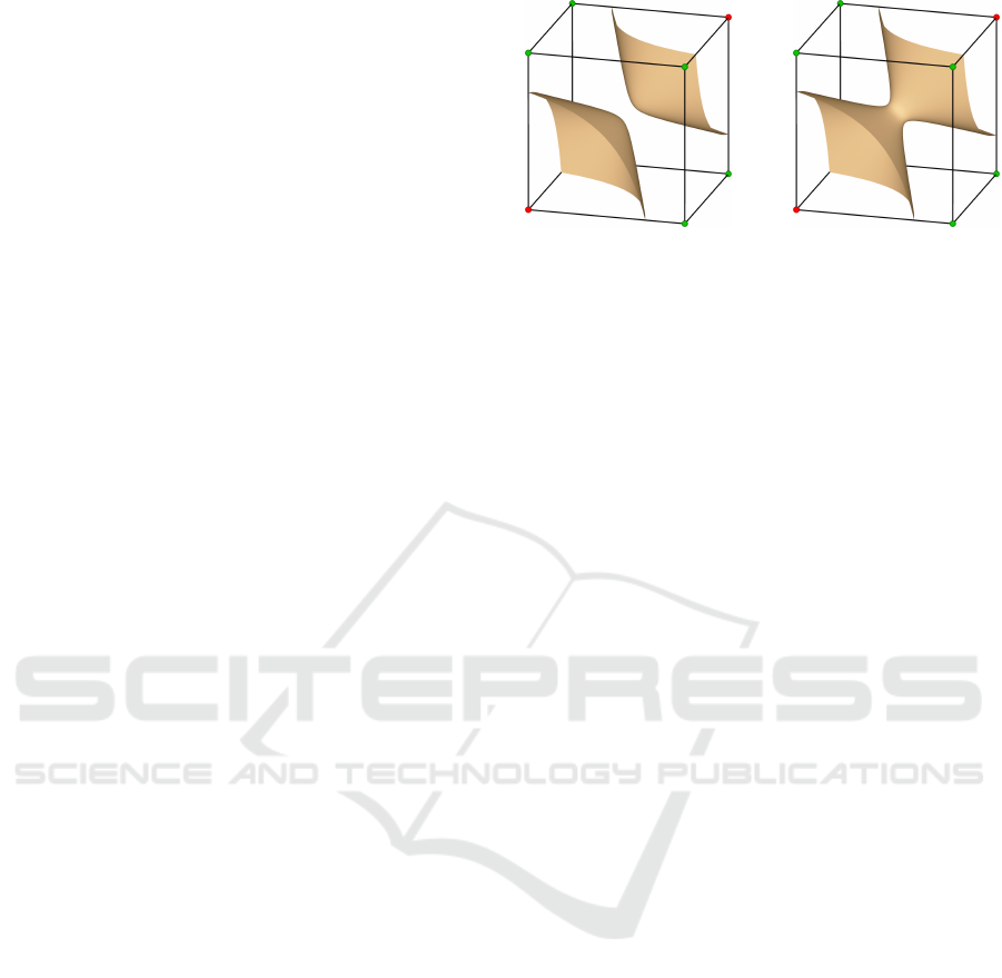
Figure 2: An interior ambiguity: the two diagonally op-

posed corners may be separated or connected by a tunnel.

(Natarajan, 1994) was the ﬁrst to describe the

problem of interior ambiguity. Here, opposite corners

of a cell can be connected by a tunnel, as shown in

Figure 2. Natarajan added four subcases to the orig-

inal 15 cases of Marching Cubes. (Chernyaev, 1996)

further extended the Marching Cubes table to include

33 different triangulations. (Etiene et al., 2012) noted

that there are cases where the triangulation of MC33

is not topologically correct. (Custodio et al., 2013)

proposed the improved version C-MC33. In (Lewiner

et al., 2012), an implementation of MC33 using mul-

tiple tables to determine subcases was discussed.

Some methods use critical points of the isosurface

to determine the topology. (Nielson, 2003) presented

an approach with multi-stage decisions that require

multiple tables. (Lopes and Brodlie, 2003) uses addi-

tional shoulder points and inﬂection points to increase

the geometric accuracy of the triangulation. (Renbo

et al., 2005) proposed a table-free variant of Lopes

and Brodlie’s method that distinguishes cases based

on the number of polygons on cell faces and inﬂec-

tion points.

(Custodio et al., 2019) presented an alternative

and table-free approach to determine the correct

topology inside a cell. They compute connected

groups of vertices and create a triangulation based on

convex hulls.

(Grosso, 2016) presented a contour-based isosur-

facing method that infers the correct topology inside a

cell from the number and conﬁgurations of isosurface

contours on cell faces. In addition, interior points are

computed for some cases and used to decide whether

a tunnel occurs. The occurrence of singular cases was

discussed in (Grosso, 2017).

Other methods rely on subdivisions to resolve

topological ambiguities. (Scheidegger et al., 2010)

used an adaptive regular subdivision scheme while

(Carr and Max, 2010) proposed subdivisions at crit-

ical points of the trilinear interpolant.(Hege et al.,

1997) proposed an algorithm that uses non-binary

classiﬁcations of the vertices and assigns them proba-

bilities for interpolation. They also subdivide the cell,

followed by a simpliﬁcation step.

GRAPP 2025 - 20th International Conference on Computer Graphics Theory and Applications

332

Another algorithm for isosurface computation is

Marching Tetrahedra (Treece et al., 1999), based on

linear interpolation within the tetrahedra. This results

in a different interpolation and therefore isosurface,

even when a hexahedral mesh is split into tetrahedra.

Recently, neural isosurfacing methods like Neural

Marching Cubes (Chen and Zhang, 2021) or Neural

Dual Contouring (Chen et al., 2022) have gained at-

tention. However, these cannot guarantee topological

correctness due to their probabilistic nature.

(Etiene et al., 2012) proposed a framework to

verify the topological properties of isosurface algo-

rithms, which we will use in Section 4 to test our

method.

3 METHOD

Table-based implementations of topologically correct

Marching Cubes require hand-crafting many individ-

ual triangulations for the different conﬁgurations of

corner values and possible topologies of a cell. There-

fore, we strive towards a universal procedural algo-

rithm based on the properties of the trilinear inter-

polant. In contrast to previous work, our method in-

cludes the topologically correct triangulation of sin-

gular cases without increasing in complexity. The

following chapter analyzes the isosurface obtained

by trilinear interpolation and describes its topologi-

cal properties. Afterward, an algorithm is presented

that leverages these insights to generate a procedu-

ral triangulation of the isosurface without relying on

lookup tables.

3.1 Topology of Trilinear Interpolation

To analyze the topology of the trilinear interpola-

tion we consider only a single unit cell for simplic-

ity. Marching Cubes assumes the values inside of a

cell to be a trilinear interpolation of the corner values

, ..., f

deﬁned as

F(u, v, w) =

(1 − u)(1 − v)(1 − w) f

+ u(1 − v)(1 − w) f

+(1 − u)v(1 − w) f

+ uv(1 − w) f

+(1 − u)(1 − v)w f

+ u(1 − v)w f

)

+(1 − u)vw f

+ uvw f

(1)

where (u, v, w) ∈ [0, 1]

are the local coordinates of the

cell. We assume w.l.o.g. that the isovalue is zero, so

the isosurface is described by

F(u, v, w) = 0. (2)

Positive values are considered to be on the outside of

the isosurface, and corners of a cell with a positive

or negative value are called positive and negative cor-

ners, respectively.

Previous work showed that the topology of the iso-

surface of a trilinear interpolation can be ambiguous

on the faces of the cell and its interior. Firstly, we

focus on distinguishing different topological cases of

the intersection of the isosurface with a face. In the

following, we consider the face w = 0 with corner val-

ues f

, f

. The restriction of Equation (1) to the

plane deﬁned by this face is the bilinear interpolation

w=0

(u, v) = (1 − v)((1 − u) f

+ u f

)

+v ((1 − u) f

+ u f

(3)

which can be written in normal form as

w=0

(u, v) = α + η(u − u

)(v − v

) (4)

with

η = f

− f

+ f

(5)

α =

− f

(6)

− f

, v

− f

. (7)

This form shows that the intersection of the isosur-

face with a plane is generally a hyperbola as shown

in Figure 3a with the asymptotes u = u

and v = v

when α ̸= 0 and η ̸= 0. However, Equation (4) can

degenerate and lead to three other topological cases

on the face that are shown in Figure 3. If α = 0 and

η ̸= 0, the hyperbola collapses to the two lines u = u

and v = v

in Figure 3b that meet at the center of the

asymptotes (u

, v

). We call a face with this topology

a singular face and the point (u

, v

) a singular point

on the face. This point is not necessarily singular in

three dimensions depending on the incident cells.

If η = 0 Equation (4) is no longer deﬁned. Instead,

the bilinear interpolation from Equation (3) degener-

ates to the linear interpolation

w=0

(u, v) = f

+ u( f

− f

) + v( f

− f

), (8)

where the solution to F

w=0

(u, v) = 0 is either a single

straight line visualized in Figure 3c or in the case f

= f

= 0 the solution is the whole plane w = 0

shown in Figure 3d.

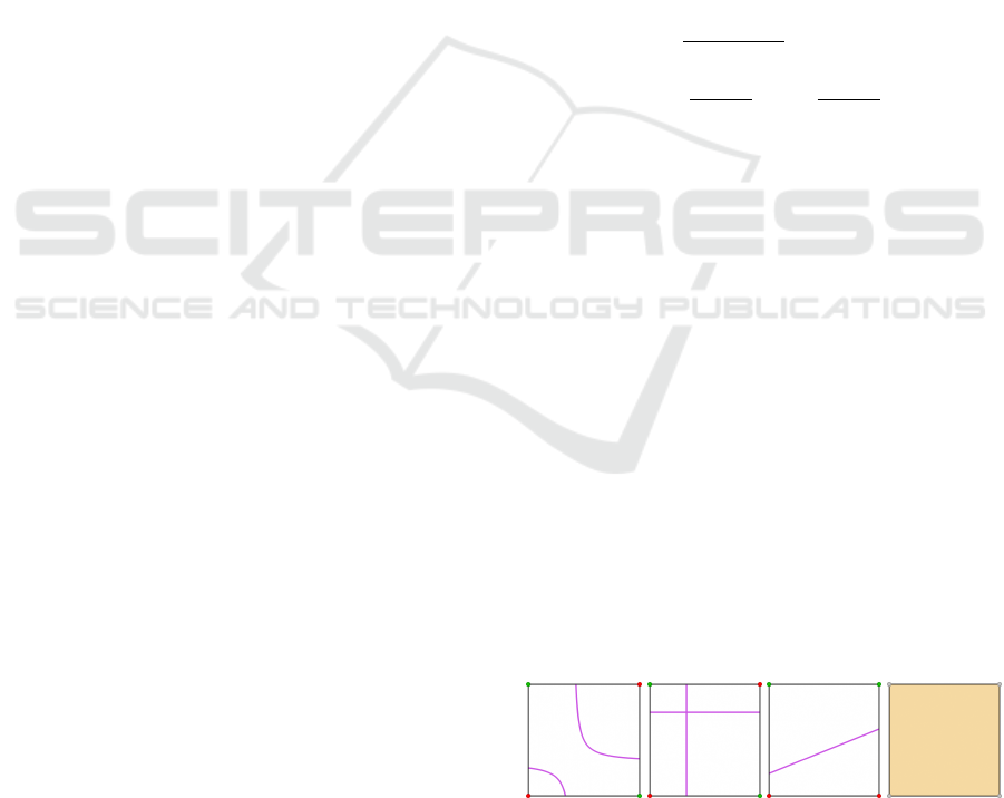
(a) hyperbola (b) cross (c) single line (d) plane

Figure 3: The topologies of the isosurface on a face.

The cases where the intersection of the isosurface

with a face is a single line or the whole plane cannot

MCPro: A Procedural Method for Topologically Correct Isosurface Extraction Based on Marching Cubes

333

be ambiguous. However, the hyperbolic and singular

cases have an ambiguous topology because they con-

sist of two branches of the isosurface. From the signs

of the values f

, ..., f

, it cannot be determined how

the two branches are oriented. In the singular case, the

two branches meet at the center of the asymptotes, but

if we move in the direction orthogonal to the surface,

the two branches will separate or merge, see Figure

10. The correct topology is deﬁned by the limit when

the face is approached from the cell’s interior.

After resolving face ambiguities, we now analyze

interior ambiguities of the trilinear interpolant. Inte-

rior ambiguities can even occur if no faces are am-

biguous. The isosurface can be described in paramet-

ric form by solving Equation (2) for one of u, v, or w,

e.g.

w(u, v) =

auv + bu + cv + d

euv + f u + gv + h

, (9)

where a, ..., h depend on the values at the cell corners

, ..., f

. We look at the critical points’ existence and

positions to determine the topology of the isosurface.

Between critical points and the cell’s boundaries, the

surface is monotonic. The surface deﬁned by w(u, v)

has up to two critical points that satisfy

∂w(u, v)

∂u

∂w(u, v)

∂v

= 0. (10)

These critical points are saddle points of the isosur-

face because the determinant of the Hessian is nega-

tive at the critical points, so minima and maxima do

not exist. The same holds for u(v, w) and v(u, w), re-

sulting in up to six critical points of the isosurface.

Because the partial derivatives in two directions are

zero, the saddle points lie on the intersections of two

axis-aligned lines that are part of the isosurface, as

shown in Figure 4a.

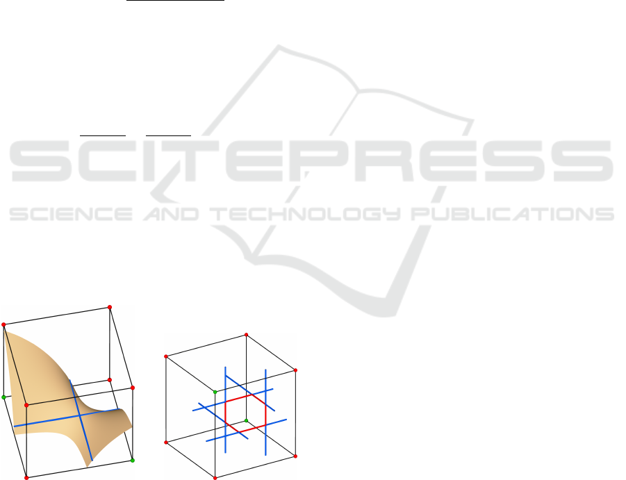
(a) (b)

Figure 4: (a) A saddle point is located at the intersection of

two axis-aligned anchor lines shown in blue. (b) The inner

hexagon marked in red consists of six critical points on the

anchor lines forming a cuboid.

We call these axis-aligned lines with constant value

anchor lines. There can be at most six of these anchor

lines. The saddle points are the same ones computed

by (Grosso, 2016) by solving three quadratic equa-

tions. The advantage of the formulation in Equation

(10) is that it is not based on the intersection of the

isosurface with cell faces that can degenerate to the

singular case. If all six critical points exist, they form

six corners of a cuboid, where two diagonally oppo-

site corners are missing. This structure is called De-

Vella’s Necklace (Nielson, 2003) or Inner Hexagon

(Grosso, 2016) and is visualized by the red lines in

Figure 4b. The case of two crossing lines, Figure 3b,

occurs precisely in the case where one or more ver-

tices of the inner hexagon lie on a face of the cell.

3.2 Triangulation Algorithm

Due to the high number of possible combinations of

cell corner values, face ambiguities, interior ambi-

guities, and singularities, storing all potential cases

of triangulations in tables is infeasible. The trian-

gulation is therefore generated procedurally based on

properties of the trilinear interpolation inside a cell.

All conﬁgurations are processed similarly without re-

lying on many execution paths for individual edge

cases. For example, cases that contain cell corners

with exactly the isovalue do not require a large in-

crease of handcrafted triangulations as proposed by

(Raman and Wenger, 2008). The algorithm is split

into four stages that analyze features of increasing di-

mensionality of the grid. This enables efﬁcient par-

allelization and reduces duplicate computations. Our

algorithm creates the triangulation based on contours

on the faces and interior of a cell. The isosurface is

represented by oriented segments stored in a halfedge

data structure that allows efﬁcient insertion and up-

dates.

The ﬁrst three stages of the algorithm are iterating

all cell edges of the grid, then the faces, and lastly,

the cells. While the edges are considered, new ver-

tices are created. When the faces are analyzed, if

the face is singular, a new vertex on the face is cre-

ated, and the vertices are connected to line segments.

While iterating the cells in the third stage, a halfedge

data structure is created by connecting the segments

to form contours, interior vertices are added, and the

interior structure is connected to the contours. In the

ﬁnal step, the halfedge data structure is triangulated

to create a mesh. In the following, the principal steps

of the algorithm are explained in more detail.

Firstly, all edges are iterated and checked for an

intersection with the isosurface. If the values at the

endpoints of an edge are on different sides of the iso-

surface, a new vertex is created at the position deter-

mined by linear interpolation. If both endpoints of an

edge lie on the isosurface, they are added to the list

GRAPP 2025 - 20th International Conference on Computer Graphics Theory and Applications

334

of vertices, and no interpolation is performed. Oth-

erwise, the edge does not intersect the isosurface and

can be ignored.

Next, the faces are considered. The intersection

of the isosurface with a plane can have four different

mathematic descriptions that are distinguished by the

asymptotic decider in Equation (6). Based on these

different topologies, the vertices on a face are con-

nected to segments. Therefore, each face is divided

into quadrants based on the center of the asymptotes

given by Equation (7). The vertices on the face are

sorted into their respective quadrants. The non-empty

quadrants must contain two vertices that are con-

nected by a segment. The singular cases can be solved

similarly by connecting all vertices on the cell’s edges

to the central, singular vertex on the face.

Because the segments are later converted to

halfedges, they must be correctly oriented. Each seg-

ment has a tangential and a normal direction, where

the normal is on the left side of the tangent. Since

we deﬁned positive values as outside the isosurface,

the normal of the line segments should always point

towards a positive corner of the face. The orienta-

tion of the segment is computed based on its normal

direction and the sign of a corner in the same quad-

rant like in Figure 5a. For singular faces, the normal

of the face at the asymptotic center is also used to

decide how the four segments are connected. Con-

nected segments must rotate counter-clockwise for a

face normal facing outwards as shown in Figure 5b.

Repeating this procedure for all faces leads to the seg-

ments in Figure 5c that represent the intersection of

the isosurface with the faces of a cell.

(a) hyperbolic face (b) singular face (c) outer contours

Figure 5: The segments on a face are connected and ori-

ented based on corner values and the face normal to form

contours.

Finally, the segments on the faces are connected to

form contours on the cell faces, and the topology of

the isosurface inside the cell is evaluated. The mesh

inside of a cell is represented by a local halfedge data

structure. The segments generated on the faces of the

cell are inserted and pointers to the next and previ-

ous halfedges are stored. Then, two opposite critical

points are computed by solving the system of equa-

tions (10). The remaining four points of the inner

hexagon shown in Figure 4b are inferred by combin-

ing the coordinates of the two known solutions. The

anchor lines and the hexagon shown in Subsection 3.1

form a skeleton inside the cell that is used to deter-

mine the triangulation. All critical points inside the

cell are added to the list of vertices. The critical points

that lie on the face coincide with the points already

calculated during the face iteration and are therefore

not added to the list. The intersections of an anchor

line with the faces of the cell will always lie on a con-

tour of the exact, trilinear isosurface as can be seen

in Figure 6a. To connect the inner hexagon with the

outer contours, segments are created from every crit-

ical point to the outer vertices according to the skele-

ton of anchor lines. However, the outer end of an an-

chor line generally does not coincide with a contour

vertex. Thus, the vertex that corresponds to the inter-

sected contour and is closest to the intersection point

with the face is chosen instead. This is repeated for

all critical points. Additionally, the segments of the

inner hexagon are added to complete the inner skele-

ton of halfedges shown in Figure 6b. The connectivity

of halfedges at the inner vertices is decided by choos-

ing the surface normal to face outward according to

the interpolated gradient of the function values at that

point. The outer contour is split at intersected ver-

tices and is newly connected to and from the inner

vertices. This way, the created halfedge data structure

describes a polygonal mesh of the isosurface.

(a) (b)

Figure 6: (a) The intersection of the anchor lines with the

faces of the cell is always on the contour of the isosurface.

(b) The contours of the isosurface inside a cell based on the

skeleton of anchor lines.

Because the isosurface is monotonic between critical

points, its topology is equivalent to a disk’s. The re-

sulting polygons described by the halfedge data struc-

ture can therefore be triangulated as disks. This is

done by iteratively replacing two incident halfedges

with the spanned triangle and inserting the third side

as a new halfedge. The resulting mesh can be output

as an indexed face set or a global halfedge data struc-

ture.

This formulation inherently solves many conﬁgu-

MCPro: A Procedural Method for Topologically Correct Isosurface Extraction Based on Marching Cubes

335

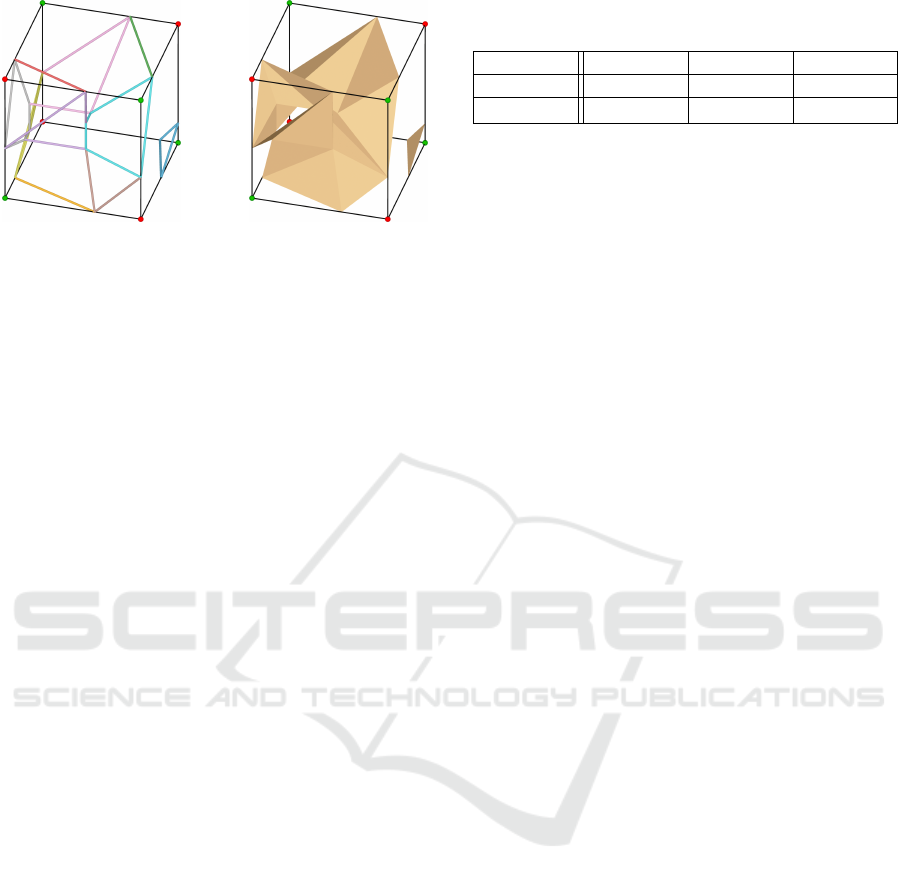
Figure 7: The halfedge data structure represents the surface

as polygons shown in different colors on the left. The poly-

gons are triangulated to create the ﬁnal mesh on the right.

rations that previous methods could only solve based

on some decision criteria for the correct topology. For

example, the normals of neighboring saddle points

decide whether a tunnel or disc is created for MC

case 13 because the halfedges will be oriented differ-

ently. From there, the same triangulation algorithm

creates the correct meshes for both topologies instead

of needing to deﬁne an explicit case distinction.

4 RESULTS

In this section, we present some results of our new

triangulation algorithm, test the method on real-world

datasets, and show some singular cases of implicitly

deﬁned surfaces for the trilinear interpolant that are

non-manifold. For comparison purposes we use the

MC33 implementation in the scikit library, (van der

Walt et al., 2014).

In contrast to previous work, we focused on the

cases where the intersection of the isosurface with a

cell face is a degenerated hyperbola. Our table-free

method generates topologically correct triangulations

compared to the trilinear interpolant. Some examples

of such cases on one or multiple faces can be seen in

Figure 8. A reference for the exact trilinear isosur-

face is obtained by subdividing each cell at least 100

times and computing the isosurface within the sub-

cells. Tunnels in the isosurface are correctly repre-

sented in the mesh created by our method, even for

the singular cases where one or more saddle points lie

on the faces of the cell. MC33 can not produce a topo-

logically correct mesh for these cases. For the middle

case in Figure 8 with three singular faces next to each

other, MC33 creates a tunnel with triangles on the

cell faces, leading to an incorrect non-manifoldness

when connected to the neighboring cells. Our use of

a halfedge data structure prevents this by describing

the face neighborhood with opposite halfedges.

We veriﬁed our algorithm with the test datasets

provided by (Etiene et al., 2012). The datasets contain

Table 1: The number of mesh elements of the human skull

(isovalue 950) created by our method, MC33, and MC.

Method Ours MC33 MC

Vertices 1213089 1102349 1093007

Triangles 2434920 2219708 2212832

10000 single-cell examples, and 10000 closed sur-

faces together with precomputed topological invari-

ants. To compare the topology of the meshes gener-

ated by our method to the trilinear interpolant, we use

Betti numbers b

(Konkle et al., 2003). Only b

, b

and b

can be non-zero in three-dimensional space.

Here, b

describes the number of connected compo-

nents. b

counts the one-dimensional holes of an ob-

ject and can be computed as b

= 2g, where g is the

genus of the surface (Theisel, 2002). The number b

represents the regions of space enclosed by the sur-

face. We additionally used the Euler characteristic

χ = V − E + F as a topological invariant for compar-

isons. Our method generates isosurfaces with the cor-

rect topology in all 20000 examples provided by the

test datasets. Note that the test datasets did not con-

tain any singular faces.

We used our algorithm to compute the isosurface

from some real-world datasets of a human skull, a

mecanix, a Porsche, and a carp, as shown in Figure 9.

CT and MRI datasets contain only 16-bit integer data

values, which increases the probability for singu-

lar faces and non-manifold cases. We analyzed 22

datasets of which all but one contain singular faces

and therefore require special handling of these cases.

Our algorithm produces a more detailed mesh be-

cause critical points are included in the triangulation.

Therefore, the number of vertices and triangles in-

creases compared to MC33. As Table 1 shows for the

example of the human skull dataset, our method gen-

erates approximately 10 % more vertices and faces

than the standard Marching Cubes and the MC33 al-

gorithms.

We now look at non-manifoldness occurring in the

trilinear interpolant. The face of a cell whose inter-

section with the isosurface is a degenerated hyperbola

contains a vertex on the face. Although the vertex is

singular on the face, it can be part of a continuous

surface through the two incident cells where the ver-

tex is not singular in three dimensions. In Figure 10,

we see on the left that the cross lies on a single branch

of the isosurface, and thus, the singular point is mani-

fold in 3D. On the other side, on the right, we see two

branches of the isosurface touch at the singular point.

The singular point corresponds to a singularity of the

implicit surface, creating a non-manifold vertex.

The previous example shows that the trilinear in-

terpolant can be singular on faces, edges, and cor-

ners, for which the topologically correct triangulation

GRAPP 2025 - 20th International Conference on Computer Graphics Theory and Applications

336

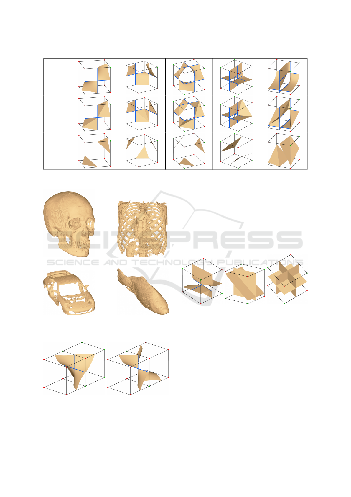
Trilinear

Ours

MC33

Figure 8: The triangulations created by subdividing and interpolating the grid values, our method, and MC33 for cases with

at least one degenerated hyperbola.

(a) Human skull (b) Mecanix

Figure 9: Meshes generated with our method from a selec-

tion of real-world datasets.

Figure 10: Two cells that share a singular face can either re-

sult in a continuous surface (left) or a singular surface with

a non-manifold vertex (right).

is non-manifold. As seen in Figure 11, Singularity

can also occur within a cell. A singular point oc-

curs if all six saddle points coincide and the tunnel

collapses to a single point in space. In this case, the

isosurface and the topologically correct triangulation

are non-manifold. The case of an isosurface, which is

non-manifold along an edge, occurs if the scalar val-

ues of the cell vertices are symmetric in such a way

that an axis-aligned plane is part of the isosurface.

Figure 11: Non-manifold vertices and edges can occur in

the trilinear interpolant.

The geometric accuracy of the triangulation of the iso-

surface within a cell can be improved by edge ﬂips for

some cases where the three-dimensional shape of the

polygons that make up the isosurface is not optimal.

The topologically correct triangulation of cases con-

taining non-manifold edges, such as in Figure 11, will

be the subject of future work.

5 CONCLUSIONS

We presented an isosurface method that generates

meshes topologically equivalent to the isosurface of

the trilinear interpolation of a scalar ﬁeld. The method

does not rely on lookup tables like many previous

MCPro: A Procedural Method for Topologically Correct Isosurface Extraction Based on Marching Cubes

337

variants of Marching Cubes. Instead, it generates the

triangulation in a procedural algorithm based on a lo-

cal halfedge data structure. The correct topology is

determined by the contours on the cell faces and the

conﬁguration of critical points inside the cell. Com-

pared to previous methods, our approach generates

topologically correct triangulations for cases where

the intersection of the trilinear interpolant and a cell

face is not hyperbolic but degenerates into two cross-

ing lines. Our method creates a more detailed mesh

by making use of critical points of the surface. We

showed that an isosurface based on trilinear interpo-

lation can be non-manifold both inside of a cell and

on the boundary between cells, so a topologically cor-

rect triangulation should include these non-manifold

features.

ACKNOWLEDGEMENTS

This work was funded by the Deutsche Forschungs-

gemeinschaft (DFG, German Research Foundation) –

502500606.

REFERENCES

Carr, H. and Max, N. (2010). Subdivision Analysis of the

Trilinear Interpolant. IEEE Transactions on Visualiza-

tion and Computer Graphics, 16(4):533–547.

Chen, Z., Tagliasacchi, A., Funkhouser, T., and Zhang, H.

(2022). Neural dual contouring. ACM Trans. Graph.,

41(4):104:1–104:13.

Chen, Z. and Zhang, H. (2021). Neural marching cubes.

ACM Trans. Graph., 40(6):251:1–251:15.

Chernyaev, E. (1996). Marching Cubes 33: Construction of

Topologically Correct Isosurfaces. No. CERN-CN-95-

17.

Custodio, L., Etiene, T., Pesco, S., and Silva, C.

(2013). Practical considerations on Marching Cubes

33 topological correctness. Computers & Graphics,

37(7):840–850.

Custodio, L., Pesco, S., and Silva, C. (2019). An extended

triangulation to the Marching Cubes 33 algorithm.

Journal of the Brazilian Computer Society, 25(1):6.

Etiene, T., Nonato, L. G., Scheidegger, C., Tienry, J., Pe-

ters, T. J., Pascucci, V., Kirby, R. M., and Silva, C. T.

(2012). Topology Veriﬁcation for Isosurface Extrac-

tion. IEEE Transactions on Visualization and Com-

puter Graphics, 18(6):952–965.

Grosso, R. (2016). Construction of Topologically Correct

and Manifold Isosurfaces. Computer Graphics Forum,

35(5):187–196.

Grosso, R. (2017). An asymptotic decider for robust

and topologically correct triangulation of isosurfaces:

topologically correct isosurfaces. Proceedings of the

Computer Graphics International Conference, pages

1–5.

Hege, H.-C., Stalling, D., Seebass, M., and Z

ockler, M.

(1997). A generalized marching cubes algorithm

based on non-binary classiﬁcations. SC-97-05.

Konkle, S. F., Moran, P. J., Hamann, B., and Joy, K. I.

(2003). Fast methods for computing isosurface topol-

ogy with betti numbers. In Data Visualization: The

State of the Art, pages 363–375.

Lewiner, T., Lopes, H., Vieira, A., and Tavares, G. (2012).

Efﬁcient Implementation of Marching Cubes’ Cases

with Topological Guarantees. Journal of Graphics

Tools, 8.

Lopes, A. and Brodlie, K. (2003). Improving the robust-

ness and accuracy of the marching cubes algorithm

for isosurfacing. IEEE Transactions on Visualization

and Computer Graphics, 9(1):16–29.

Lorensen, W. E. and Cline, H. E. (1987). Marching cubes:

A high resolution 3D surface construction algorithm.

In Proceedings of the 14th annual conference on

Computer graphics and interactive techniques, SIG-

GRAPH ’87, pages 163–169.

Natarajan, B. K. (1994). On generating topologically con-

sistent isosurfaces from uniform samples. The Visual

Computer, 11(1):52–62.

Newman, T. S. and Yi, H. (2006). A survey of the marching

cubes algorithm. Computers & Graphics, 30(5):854–

879.

Nielson, G. (2003). On Marching Cubes. IEEE Trans-

actions on Visualization and Computer Graphics,

9:283–297.

Nielson, G. and Hamann, B. (1991). The asymptotic de-

cider: resolving the ambiguity in marching cubes. In

Proceeding Visualization ’91, pages 83–91.

Nielson, G., Huang, A., and Sylvester, S. (2002). Approxi-

mating normals for marching cubes applied to locally

supported isosurfaces. In IEEE Visualization, 2002.

VIS 2002., pages 459–466.

Raman, S. and Wenger, R. (2008). Quality Isosur-

face Mesh Generation Using an Extended Marching

Cubes Lookup Table. Computer Graphics Forum,

27(3):791–798.

Renbo, X., Weijun, L., and Yuechao, W. (2005). A Robust

and Topological Correct Marching Cube Algorithm

Without Look-Up Table. In The Fifth International

Conference on Computer and Information Technology

(CIT’05), pages 565–569.

Scheidegger, C., Etiene, T., Nonato, L. G., and Silva, C. T.

(2010). Edge Flows: Stratiﬁed Morse Theory for Sim-

ple, Correct Isosurface Extraction. SCI Institute, Uni-

versity of Utah, SCI Technical Report UUSCI-2010-

002.

Stahl, J. (2025). MCPro [Software]. Github.

https://github.com/JulyCode/MCPro.

Theisel, H. (2002). Exact Isosurfaces for Marching Cubes.

Computer Graphics Forum, 21(1):19–32.

Treece, G. M., Prager, R. W., and Gee, A. H. (1999). Regu-

larised marching tetrahedra: improved iso-surface ex-

traction. Computers & Graphics, 23(4):583–598.

van der Walt, S., Sch

onberger, J. L., Nunez-Iglesias, J.,

Boulogne, F., Warner, J. D., Yager, N., Gouillart,

E., Yu, T., and the scikit-image contributors (2014).

scikit-image: image processing in Python. PeerJ,

2:e453.

GRAPP 2025 - 20th International Conference on Computer Graphics Theory and Applications

338