Implementing the Perturbation Approach for Reliability Assessment: A
Case Study in the Context of Flight Delay Prediction
Simon Staudinger
a
, Christoph Großauer, Pascal Badzura, Christoph G. Schuetz
b
and Michael Schrefl
c
Keywords:
Business Intelligence, Data Mining, Predictive Analytics, Air Traffic Management.
Abstract:
Organizations employ prediction models as a foundation for decision-making. A prediction model learned
from training data is often only evaluated using global quality indicators, e.g., accuracy and precision. These
global indicators, however, do not provide guidance regarding the reliability of the prediction for a specific
input case. In this paper, we instantiate a generic reference process for implementing reliability assessment
methods for specific input cases on the real-world use case of flight delay prediction. We specifically imple-
ment the perturbation approach to reliability assessment for this use case and then describe the steps that were
taken to train the prediction model, with an emphasis on the activities required to implement the perturbation
approach. The perturbation approach consists of slightly altering feature values for an individual input case,
e.g., within the margins of error of a sensed value, and observe whether the prediction of the model changes,
which would render the prediction unreliable. The implementation of the perturbation approach requires de-
cisions and documentations along the various stages of the data mining process. A generic tool can be used to
document and perform reliability assessment using the perturbation approach.
1 INTRODUCTION
Organizations employ prediction models in various
domains to obtain predictions regarding future events,
which can be used to determine the best course of
action for the organization (Siegel, 2013). Typical
metrics for model evaluation, e.g., accuracy and pre-
cision, provide an impression of the overall, average
performance of the model. Such global metrics, how-
ever, do not necessarily reflect the reliability of a spe-
cific prediction for a certain input case, i.e., a combi-
nation of feature values, since the input case may re-
semble cases from the training data where the model
routinely failed to accurately predict the outcome.
Assessing the reliability of an individual predic-
tion for a specific input case is crucial if an organi-
zation intends to use that prediction as the basis for
decisions. To this end, a reference process for imple-
menting specific methods for reliability assessment in
the context of data mining projects has been proposed
by Staudinger et al. (2024). This reference process
a
https://orcid.org/0000-0002-8045-2239
b
https://orcid.org/0000-0002-0955-8647
c
https://orcid.org/0000-0003-1741-0252
is organized along the Cross-Industry Standard Pro-
cess for Data Mining (CRISP-DM) and can be instan-
tiated for specific prediction problems as well as spe-
cific methods for reliability assessment.
The perturbation approach is a specific method
for reliability assessment. Feature values of input
cases can be imprecise as a consequence of how data
are collected or prepared. For example, sensor im-
precision in data collection or numerosity reduction
in data preparation may cause captured feature values
to deviate from the actual value. To assess the reli-
ability of an individual prediction, knowledge about
the domain, the input features, and the preprocessing
steps of the features is necessary to determine the ad-
missible range within which the value captured in the
data may deviate from the actual value. The predic-
tion should not change for a specific input case if the
feature values are changed (“perturbed”) within the
admissible range.
Apart from imprecision in the collected and pre-
processed data, the existence of edge cases may also
lead to unreliable predictions, which could likewise
be spotted by perturbation of input features. If a
small change in an input feature causes the prediction
to change, the case may be an edge case where the
Staudinger, S., Großauer, C., Badzura, P., Schuetz, C. G. and Schrefl, M.
Implementing the Perturbation Approach for Reliability Assessment: A Case Study in the Context of Flight Delay Prediction.
DOI: 10.5220/0013299700003929
Paper published under CC license (CC BY-NC-ND 4.0)
In Proceedings of the 27th International Conference on Enterprise Information Systems (ICEIS 2025) - Volume 1, pages 75-86
ISBN: 978-989-758-749-8; ISSN: 2184-4992
Proceedings Copyright © 2025 by SCITEPRESS – Science and Technology Publications, Lda.
75

prediction model produces results that are unreliable,
which can be factored into the decisions based on the
predictions.
In this paper, we implement the perturbation ap-
proach for reliability assessment of flight delay pre-
dictions by instantiating the generic reference pro-
cess for implementing reliability assessment meth-
ods of predictive analytics results in data mining
projects (Staudinger et al., 2024). During the develop-
ment of a prediction model, we collect metadata about
the admissible ranges of features during the business
understanding, data understanding, and data prepro-
cessing stages of the CRISP-DM, and we determine
perturbation options for each feature of an input case
during the modeling stage. After the deployment of
the developed prediction model, analysts can apply
perturbation using the previously identified perturba-
tion options to assess the reliability of an individual
prediction for a given input case.
We use the real-world case of flight delay predic-
tion, inspired by the work of Bardach et al. (2020), to
demonstrate the practical applicability and usefulness
of the perturbation approach. Flight delay predictions
can be used to counter the negative consequences of
delays by swapping departure/arrival slots of flights
early on (Lor
¨
unser et al., 2021), and information re-
garding the reliability of the delay prediction for an
individual flight can be factored into the decision to
swap slots. Using perturbation, the reliability of the
prediction of a flight delay could be checked. A de-
lay prediction detected to be unreliable might then
not be used as the basis for deciding to swap flights
or a human expert with extensive domain experience
may look more closely at the flight to manually deter-
mine whether the prediction is likely correct, possibly
based on additionally collected data.
The perturbation approach for reliability assess-
ment of individual predictions is similar to sensitiv-
ity analysis (Pianosi et al., 2016), where the aim is to
find important features that have a considerable influ-
ence on the prediction by consecutively perturbing all
of the input values. In contrast to sensitivity analy-
sis, however, we perturb individual input values for a
specific input case based on information gathered dur-
ing the development of the prediction model to assess
whether possible inaccuracies of the input values may
lead to a changed prediction. A changed prediction
would then raise suspicions regarding the reliability
of the prediction.
The main contributions of this paper are as fol-
lows:
1. We demonstrate how to implement the perturba-
tion approach for a real-world use case, namely
flight delay prediction.
2. We evaluate the usefulness of applying the pertur-
bation approach to reliability assessments in the
context of the real-world use case.
3. We present a generic tool that assists analysts with
conducting the perturbation approach, eliminating
the need to re-implement basic steps of the pertur-
bation approach for different use cases.
While the development of a novel prediction model
for flight delay prediction was not the primary goal
of this paper, we nevertheless require such a model
to assess the reliability of the predictions made by a
prediction model for a given input case in order to
demonstrate the benefits of evaluating predictive re-
sults using the perturbation approach. Hence, we also
developed multiple prediction models for flight delay
prediction using real-world data.
The remainder of this paper is structured as fol-
lows. Section 2 reviews related work. Section 3 de-
scribes the development of a prediction model, with
a specific focus on design decisions and capturing of
information required for implementing the perturba-
tion approach. Section 4 examines the usefulness of
the perturbation approach in reliability assessment of
flight delay predictions. Section 5 presents a tool to
support analysts with applying the perturbation ap-
proach. Section 6 concludes with a summary and an
outlook on future work.
2 RELATED WORK
Carri
´
o et al. (2014) describe a collection of methods
that can be used to assess the reliability of the pre-
dictions of drug properties. These methods aim to as-
sess the applicability domain of a chosen model and
are grouped into three families: training set compar-
ison, activity spaces, and model perturbation. The
authors provide a software package in the R program-
ming language
1
, which takes as input the compound
molecular descriptors as well as the predicted value
and provides a single score, ranging from 0 to 6, as the
output, indicating reliability of the predicted value.
Metamorphic testing (Chen et al., 2018) is a
method known from software testing to verify the be-
havior of a software function. A metamorphic relation
describes how a change of an input value should af-
fect the respective output of the software. If the real
output is different from the one that was expected by
the metamorphic relation, the software may not work
correctly. Yang and Chui describe a reliability assess-
ment method that makes use of metamorphic testing
in the hydrological domain (Yang and Chui, 2021).
1
https://www.r-project.org/
ICEIS 2025 - 27th International Conference on Enterprise Information Systems
76

Sensitivity analysis (Pianosi et al., 2016) is used
to assess how the change of an output variable can be
mapped to the change of the input variables, which
were used to generate the output variable. For exam-
ple, to answer a question regarding what input vari-
able caused the biggest change in the output variable,
a simple form of sensitivity analysis may also employ
perturbations for the task of ranking input features ac-
cording to their importance to the respective output
and the task of screening for features with negligible
influence on the output.
3 DEVELOPMENT
The development stages of the reference process cor-
respond to the development stages of the CRISP-
DM (Wirth and Hipp, 2000): data understanding,
data understanding, data preprocessing, modeling,
and evaluation. In the following, we describe these
stages. For each stage, we first describe the general
tasks and the information attributed to flight delay
prediction according to CRISP-DM. In addition, we
then describe for each stage all the tasks and informa-
tion of interest for the reliability assessment.
3.1 Business Understanding
During business understanding, the overall goals of a
data mining project are settled and a general project
plan is made. Flight delays are a major problem
for airports and airlines and ultimately cause enor-
mous costs, ranging from 32 C for the first minute
to 80 270 C for over 300 minutes of delay per flight
(Bardach et al., 2020). In our case of predicting flight
delays, it is therefore important to know when a flight
will arrive at the airport in order to be able to re-
act to possible delays as quickly as possible to save
additional delay costs. The data mining goal of the
project was to create a predictor which is able to pre-
dict whether a specific flight will be on time, too early,
or too late.
Regarding reliability assessment, during business
understanding, the reference processes recommends
to specify the approach(es) that might be fruitful for
the reliability assessment of individual cases. We re-
viewed the initial information of the project to see if a
perturbation approach would be applicable in this use
case. Without a deeper data understand, we already
know that the input data that are used for the are is
tabular data. A perturbation approach can be applied
to tabular data, so this does not contradict the use of
perturbation in our use case. Further, as highlighted
by Bardach et al. (2020), the main reasons for the de-
lay in 2018 where due to staffing and weather. Ac-
cording to the Network Manager Annual Report from
EUROCONTROL, weather is still an issue for delays
in 2023: ”Still, disappointingly bad weather hit oper-
ations much harder in summer 2023 than in 2022 and
contributed significantly to the overall delays.” (EU-
ROCONTROL, 2024). Since weather data are consid-
ered one of the main reasons for the delay and most
of the weather data is measured using some kind of
sensor, for example, temperature or wind sensor, per-
turbing weather features within sensor precision inter-
vals looks promising for the assessment of individual
predictions. We decided, that a perturbation approach
might be applicable as reliability assessment in our
use case and proceeded further following the refer-
ence process.
3.2 Data Understanding
In the second stage, the data understanding, all data
that could have an influence on the arrival time of a
flight is collected. We are interested in data related
to the Atlanta airport in the time period of the year
2017. These data contain information about previ-
ous flights, aircraft information, Notices to Air Mis-
sion (NOTAMs), and weather information. We reused
some of the data which were collected by Bardach
et al. (2020) and will provide the original sources
for the data. The flight data was published by the
U.S. Bureau of Transportation Statistics (Bureau of
Transportation Statistics, 2024). The flight data con-
tains 28 different attributes, like the destination of
the flight, the origin of the flight, or the tail num-
ber of the operating aircraft. Weather information
was collected from the Iowa Environmental Mesonet
(IEM) (Iowa State University, 2024). The IEM pro-
vides a script in the R programming language that
can be used to retrieve weather information, e.g., air
temperature, wind speed, or cloud coverage level, for
a provided Federal Aviation Administration (FAA)
identifier. The FAA identifier is a three-character long
identifier of aviation-related facilities within the USA.
Aircraft information was retrieved from the FAA’s
Aircraft Characteristics Database (Federal Aviation
Administration, 2024). The aircraft information con-
tain technical data about an aircraft used for a specific
flight, e.g., the parking area, the tail height, or the
approaching speed. A NOTAM is a semi-structured
short message, which contains important information
that may affect a flight route or other location rele-
vant for air traffic, e.g., an airport and its infrastruc-
ture. Possible messages can be about route changes,
runway obstructions, or status reports of navigation
aids. NOTAMs are sent to ground personnel or air-
Implementing the Perturbation Approach for Reliability Assessment: A Case Study in the Context of Flight Delay Prediction
77

craft crews. Consider the following example of such a
NOTAM, where (A) depicts the reporting facility, (B)
the location of occurrence, (C) a keyword to which the
message belongs, (D) the actual message, and (E) the
effective and expiration dates (YYMMDDhhmm):
(A)!ATL 01/024 (B)ATL (C)RWY (D)10/28 CLSD
(E)1701050430-1701051130
The employed NOTAM dataset contains 16 163
NOTAMs relevant for Atlanta airport in a time win-
dow from December 2016 to January 2018.
Regarding reliability assessment, we documented
all information which may give us an indication for
unreliable predictions after deployment of the model.
One possible group of information that an analyst
can look for during data understanding is if data was
somehow captured from the real world and it is not
clear whether the captured data and the real world
data is 100% identical. This happens, for example,
when any kind of sensor is used for the determina-
tion of feature values. Normally, the sensor points
out a specific precision or accuracy, within which the
measured value deviates from the real world value. In
our flight delay prediction use case we noticed that
this was the case for all the weather data which we
took from IEM. The IEM provides detailed informa-
tion about the sensor precisions which were used to
capture the weather data
2
. The root mean squared er-
ror (RMSE) of the temperature sensor is given with
0.9 °F and 1.1 °F for the dew point temperature. The
accuracy of the wind speed sensor is given with “± 2
knots or 5% (whichever is greater)”. The accuracy
of the wind direction is given with ± 5 degrees. The
accuracy of the pressure sensor is given with ± 0.02
inches of mercury. The accuracy of the visibility sen-
sor is given with ± 0.25 miles. We documented the
information about the weather sensors for later use in
the reliability assessment.
3.3 Data Preprocessing
In the third stage, the data preprocessing, all data that
is relevant for the delay prediction is processed such
as they are suitable to be used as training data for the
machine learning models. Each of our four different
data sources has its unique characteristics and there-
fore poses special preprocessing needs, for example,
to address certain quality issues. For example, for the
flight data, the arrival day and the arrival time were
transformed to a sine/cosine representation (cyclical
encoding) to correctly encode time distances. Fur-
ther, if a flight goes past midnight, this has to be taken
into account for the calculation of the travel time. In
2
https://www.weather.gov/media/asos/aum-toc.pdf
order to get the operating aircraft for a flight, the air-
craft type needs to be joined to each flight using the
tail number included in the flight data. The tail num-
ber is similar to the license plate of a car and can be
used to identify the type of the aircraft. Information
about aircraft characteristics where taken from Air-
fleets
3
. NOTAMs may contain a wide variety of in-
formation. A lot of this information may not have any
influence on the punctuality of a flight and, therefore,
we decided to filter the NOTAMs to keep only mes-
sages that relate to airport runways. The last step of
preprocessing is to consolidate the data from the four
different sources into one single data table. We further
applied a low-variance filter and a high-correlation fil-
ter on the consolidated data table to eliminate features
that contain either very little (low variance within the
feature values) or similar (high correlation compared
to other feature(s)) information.
Regarding reliability assessment, we documented
all information that might provide further insights
for a possible perturbation assessment. For example,
while scraping and joining the aircraft characteristics
to the respective flights, we noticed that the given air-
craft type may have different subtypes with varying
characteristics. Table 1 shows an excerpt from the
technical data of various subtypes of a Boeing 737
where the wingspan of the respective aircraft varies
from 93 ft to 112.6 ft. Even if there are several years
between the introduction of different subtypes of an
aircraft type, the average service life of an aircraft is
more than 20 years, so that more than one subtype is
used at the same time. The flight data only indicates
the general aircraft type but does not mention the spe-
cific subtype of the aircraft. If specific aircraft charac-
teristics are used within a prediction model, the differ-
ences between the subtypes should be taken into ac-
count, for example, by perturbing these values within
the possible ranges. The information that can be con-
tained in NOTAMs is very diverse and ranges from
the closure of an entire runway at an airport to in-
formation about failed lights at the airport. For our
prediction model, we have decided to encode only in-
formation concerning the Atlanta runways as a fea-
ture in the training dataset. This constructed feature
has a range from 0 to 1, where the value 0 indicates
that all five runways are without a report from the
NOTAMs and 1 indicates that there is a report from
the NOTAMs for all five runways. The intermediate
feature values are realized in steps of 0.2, i.e. a value
of 0.4 would mean that there is a message for 2 run-
ways. As this value has no direct indication of the
severity of the existing message, this feature may be a
good candidate for potential perturbations.
3
https://www.airfleets.net/home/
ICEIS 2025 - 27th International Conference on Enterprise Information Systems
78

Table 1: Dimensions of Various Boeing 737 Models.
Model Wingspan Length MTOW
737-200 93.0 100.2 115 500
737-300 94.8 109.6 139 500
737-400 94.8 119.6 150 000
737-500 94.8 101.8 136 000
737-600 112.6 102.5 144 500
737-800 112.6 129.5 174 200
737-900 112.6 138.2 187 700
3.4 Modeling
In the fourth stage, the modeling, we trained three dif-
ferent machine learning models on the 31 features of
the training data with the aim to classify a flight in one
of the three classes: too early, on time, or too late.
The three models we used are a random forest clas-
sifier, a gradient boosting classifier and an adaptive
boosting classifier. The baseline to which we compare
the performance of the models is, on the one hand,
random guessing of one of the three classes, yielding
an accuracy of 43%, as well as, on the other hand,
simply adding the departure delay to the expected ar-
rival time yielding, an accuracy of 65%. Table 13 de-
picts the accuracy and precision scores of the three
models on the test data set. For the random forest
classifier, the overall accuracy is 73.43% with a pre-
cision of 58.30% for the too early class, a precision
of 78.22% for the on time class, and a precision of
88.78% for the too late class. For the gradient boost-
ing classifier, the overall accuracy is 75.19% with a
precision of 65.86% for the too early class, a precision
of 75.88% for the on time class, and a precision of
89.50% for the too late class. For the adaptive boost-
ing classifier, the overall accuracy is 71.46% with a
precision of 59.07% for the too early class, a preci-
sion of 72.30% for the on time class, and a precision
of 89.01% for the too late class.
Regarding reliability assessment, we implemented
14 different perturbation options, based on the infor-
mation that was gathered during business understand-
ing, data understanding, and data preprocessing. A
perturbation option mainly consists of an algorithm
which describes how to alter an original input value
and returns a list of these altered/perturbed values
for the original input value (Staudinger et al., 2024).
We have used two different variants of perturbation
options. The first variant is a percentage perturba-
tion (sensorPrecision), whereby the original value is
increased or decreased by a percentage. The sec-
ond variant is a step-by-step perturbation (amountIn-
Steps), whereby the original value is increased or de-
creased by a defined absolute value. Each perturba-
tion option includes the name of the option, the scale
of the feature for which it can be used, the name of the
feature which should be perturbed, possible parame-
ters like the percentage value, and a perturbation level
which indicates the severity of a changed prediction
based on perturbed values from this option. For the
perturbation level the levels red and orange are used,
whereby red means that the prediction should not be
trusted if a perturbed value from this option changes
the prediction and orange means that a changed pre-
diction may come through the change in the perturbed
value but does not affect the original prediction. We
used these two variants of perturbation options on the
following features:
Table 2: %-Perturbation Option for Temperature.
Perturbation Option
Name: sensorPrecision
Scale of Feature cardinal
Perturbed Feature: TEMP
Additionally required values: sensorPrecision%
= 1.345%
Perturbation Level: red
Based on the findings from the data understanding
phase, we know that the temperature sensor has an
RMSE of 0.9 °F. We calculated the percentage change
in the median temperature based on this RMSE using
Equation 1 and took this as the percentage value for
the perturbation.
∆
%
= (1 −
Median Temperature–RMSE
Median Temperature
) × 100
(1)
The median temperature in the respective time frame
was 66.9 °F and thus yielded a percentage of 1.345%.
Since this perturbation is based on a measurement in-
accuracy and any value within this precision inter-
val should not change the prediction, the perturbation
level for this option is set to red. The summarized
properties of the perturbation option for the tempera-
ture are shown in Table 2.
For the dew point temperature we follow the same
approach as for the temperature. The RMSE for the
dew point temperature sensor documented in data un-
derstanding was 1.1 °F. Together with a median dew
point temperature of 57 °F in the respective time
frame, Equation 1 resulted in a percentage of 1.93%.
For the wind sensor, we have documented the in-
formation in data understanding that the values were
captured inaccurately by either 5% or ± 2 knots,
which is equal to 3.704 km/h. The perturbation lev-
els for the two wind-speed perturbation options are
indicated to be red because the perturbation options
are based on sensor inaccuracies, which should not
Implementing the Perturbation Approach for Reliability Assessment: A Case Study in the Context of Flight Delay Prediction
79

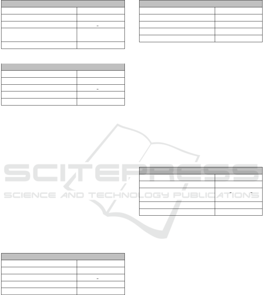
Table 3: %-Perturbation Option for Wind Speed.
Perturbation Option
Name: sensorPrecision
Scale of Feature cardinal
Perturbed Feature: WIND SPEED
Additionally required values: sensorPrecision%
= 5%
Perturbation Level: red
Table 4: Stepwise-Perturbation Option for Wind Speed.
Perturbation Option
Name: amountInSteps
Scale of Feature cardinal
Perturbed Feature: WIND SPEED
Additionally required values: amount = 3.704
Perturbation Level: red
lead to a changed prediction. The percentage pertur-
bation option for the wind speed is summarized in
Table 3 and the stepwise perturbation option for the
wind speed is summarized in Table 4.
For the humidity feature, we used the accuracy
information for the temperature and the dew point
temperature, documented in the data understanding.
Based on these accuracy information we used a for-
mula to approximate the possible deviation of the in-
dicated humidity values. We are omitting the expla-
nation of the exact approximation process of the ac-
curacy of the humidity values at this point, since this
is not decisive for the aim of this work. As result we
calculated an inaccuracy of 5.445% or 3.9498 abso-
lute, and the larger value of the both will be used in
the further assessment process. The perturbation lev-
els for the two humidity perturbation options are indi-
cated with red as they are based on sensor inaccura-
cies which should not lead to a changed prediction.
Table 5: Stepwise-Perturbation Option for Wind Direction.
Perturbation Option
Name: amountInSteps
Scale of Feature cardinal
Perturbed Feature: WIND DRCT
Additionally required values: amount = 5
Perturbation Level: red
For the wind direction sensor, we have docu-
mented the information in data understanding that the
wind direction values were captured inaccurately by
± 5 degrees. The perturbation level for the wind di-
rection perturbation option is indicated with red as it
is based on a sensor inaccuracy which should not lead
to a changed prediction. The summarized properties
of the perturbation option for the wind direction are
shown in Table 5.
Table 6: Stepwise-Perturbation Option for Runways.
Perturbation Option
Name: amountInSteps
Scale of Feature ordinal
Perturbed Feature: RUNWAYS
Additionally required values: amount = 0.2
Perturbation Level: orange
During data preprocessing, we documented that
due to the heterogeneity of the NOTAMs we only
encoded whether there was any message for one of
the runways. Thus we define a perturbation option
which alters the feature value as if there would be
one more/less runway with a mention in a NOTAM.
We have assigned orange as the perturbation level. If
a perturbed value of this runway feature would have
an effect on a specific prediction, then the respective
NOTAMs should be examined more closely. Based
on the actual content of the NOTAM information it
can be decided whether a changed prediction due to a
perturbed runway value might pose a problem for the
reliability of the prediction. The perturbation option
of the runway feature is summarized in Table 6.
Table 7: Stepwise-Perturbation Option for Sea Level Pres-
sure.
Perturbation Option
Name: amountInSteps
Scale of Feature cardinal
Perturbed Feature: SEA LEVEL
PRESSURE
Additionally required values: amount = 0.7
Perturbation Level: red
For the sea level pressure sensor, we have docu-
mented the in information in data understanding that
the pressure values were captured inaccurately by 0.7
millibar. Thus we added a perturbation option for the
sea level pressure feature which perturbs a pressure
value by this inaccuracy of 0.7 millibar. The pertur-
bation level for the sea level pressure perturbation is
indicated with red as it is based on a sensor inaccu-
racy which should not lead to a changed prediction.
Table 7 summarizes the properties of the perturbation
option for the sea level pressure.
For the precipitation per hour, we have docu-
mented the information in data understanding that the
captured precipitation has an accuracy of ± 0.02 inch.
The perturbation level for the precipitation perturba-
tion option is indicated with red as it is based on a
sensor inaccuracy which should not lead to a changed
prediction.
For the visibility, we have documented the infor-
mation in data understanding that the captured visibil-
ICEIS 2025 - 27th International Conference on Enterprise Information Systems
80

Table 8: Stepwise-Perturbation Option for Visibility.
Perturbation Option
Name: amountInSteps
Scale of Feature cardinal
Perturbed Feature: VISIBILITY
Additionally required values: amount = 0.25
Perturbation Level: red
ity has an accuracy of ± 0.25 miles. The perturbation
level for the visibility perturbation option is indicated
with red as it is based on a sensor inaccuracy which
should not lead to a changed prediction. The sum-
marized properties of the perturbation option for the
visibility are shown in Table 8.
Table 9: %-Perturbation Option for Approach Speed.
Perturbation Option
Name: sensorPrecision
Scale of Feature cardinal
Perturbed Feature: APPROACH
SPEED
Additionally required values: sensorPrecision%
= 1.4%
Perturbation Level: orange
Table 10: %-Perturbation Option for Tail Height.
Perturbation Option
Name: sensorPrecision
Scale of Feature cardinal
Perturbed Feature: TAIL HEIGHT
Additionally required values: sensorPrecision%
= 2%
Perturbation Level: orange
Table 11: %-Perturbation Option for Parking Area.
Perturbation Option
Name: sensorPrecision
Scale of Feature cardinal
Perturbed Feature: PARKING AREA
Additionally required values: sensorPrecision%
= 3%
Perturbation Level: orange
For the approach speed, the tail height, and the
parking area, we have documented the information in
data preprocessing, that based on the aircraft subtype
the characteristics of the aircraft type are different. In
general, it would be possible to determine the respec-
tive aircraft type for each new input case and perturb
the aircraft characteristics based on the different data
of the aircraft subtypes. However, since there are a
large number of different aircraft types and a list of all
aircraft subtypes must always be maintained, we have
decided to perturb the aircraft characteristics based on
median numerical distance to closest neighbor group
in the training data set. The calculations yielded a me-
dian distance of 1.4% for the approach speed, a 2%
for the tail height, and a 3% deviation for the parking
area. We assigned the perturbation level orange for
perturbation options of aircraft characteristics, mean-
ing that a changed prediction due to a perturbed value
of a respective perturbation option should be further
assessed by a human and does not automatically indi-
cate an unreliable prediction. Table 9 summarizes the
perturbation option for the approach speed, Table 10
summarizes the perturbation option for the tail height,
and Table 11 summarizes the perturbation option for
the parking area.
In the fifth stage—the evaluation—the assessment
whether the results from the modeling step fulfill the
criteria defined in business understanding is done.
This assessment includes a review of previous taken
steps and the next steps towards deployment or re-
vision of the model are discussed. We do not want
to discuss the evaluation stage of the assessment ap-
proach further within this paper and leave the discus-
sion whether to create or remove perturbation options
or to adjust parameter values for already existing per-
turbation for future work.
4 DEPLOYMENT
In the CRISP-DM, the developed prediction model is
loaded into the production system during the deploy-
ment phase and needs to be monitored further. We
first describe the general procedure of perturbation
assessment after deployment of a model using an il-
lustrative example before presenting the results of the
perturbation assessment used within the flight delay
prediction use case.
4.1 Reliability Assessment
Table 12 illustrates an example of a reliability assess-
ment. The first row shows an input case for a specific
flight, which the model predicted to arrive on time.
In data understanding, we have determined that
the Wind Direction was captured with a precision of
± 5 degrees. Therefore, we perturb the Wind Direc-
tion feature by 5 degrees, as shown in Rows 2 and 3,
and we received the same prediction as for the input
case, which thus offers no reason to characterize the
prediction as unreliable.
We also know that the sensor that was used to
measure the Wind Speed had a sensor precision of
± 3.704% km/h that the measured value may devi-
Implementing the Perturbation Approach for Reliability Assessment: A Case Study in the Context of Flight Delay Prediction
81

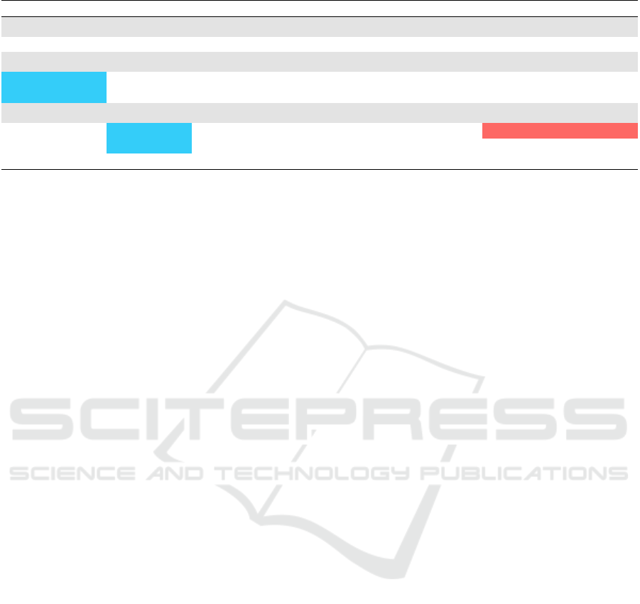
Table 12: Illustrative example of a reliability assessment.
Wind Direction Wind Speed Temperature Parking Area Tail Height ... Delayed(predicted class)
Input Case:
70 22.22 27.77 1525.18 9 ... on time
Wind Direction perturbed:
75 22.22 27.77 1525.18 9 ... on time
65 22.22 27.77 1525.18 9 ... on time
Wind Speed perturbed:
70 25.924 27.77 1525.18 9 ... too late
70 18.516 27.77 1525.18 9 ... on time
... ... ... ... ... ... ...
ate from the actual value, it would be advisable to
check multiple values within the ± 3.704% range of
sensor precision around the measured value. In the
illustrative example we obtained two perturbed cases
by adding and subtracting the 3.704 km/h to the orig-
inal feature value of the Wind Speed, as shown in the
rows 4 & 5. One of these perturbed test cases (row 4)
have a changed prediction compared to the prediction
of the input case. Since we do not know the exact
value of the Wind Speed within the range of the sen-
sor precision, the prediction should not change when
using any other value within that range. Thus, the ob-
served case should be marked as unreliable and for-
warded to a domain expert for further examination.
4.2 Results
After development, when the model is deployed into
production, including all perturbation options, every
new input case’s reliability can be assessed using the
results from the perturbation approach. In this paper
we evaluate the perturbation approach based on the
test data which were used for the calculation of the
performance metrics of the prediction model. The test
data consists of 65 801 input cases. During modeling,
we trained three different prediction models, namely,
random forest classifier, gradient boosting classifier,
and adaptive boosting classifier, the performance met-
rics of which are shown in the first row of the respec-
tive segment in Table 13. These performance metrics
are used as baseline and we now further examine to
what extent the perturbation approach might be able
to improve these metrics.
We use two metrics regarding the perturbation ap-
proach. First, we calculate the potential accuracy that
could be achieved with reliability assessment using
the perturbation approach under the assumption that
a human expert were able to determine the correct
prediction for each unreliable input case. Second,
we calculate the ratio between the increase in accu-
racy when a human expert were able to determine
the correct prediction for unreliable input cases de-
tected using the perturbation approach compared to
the increase in accuracy when looking at randomly
selected input cases. An input case is considered as
unreliable if there is at least one perturbed test case
with a changed prediction from the prediction model
compared to the original input case that does not con-
tain any perturbed values. For the evaluation of the
perturbation approach we are only considering single-
feature perturbations, i.e., we are only perturbing sin-
gle features and do not consider the combination of
more than one perturbed feature.
Considering the random forest classifier, using the
perturbation options described in Section 3, we found
7 249 unreliable input cases. Thus, 11.01% (7 249
÷ 65 801) of all test cases were marked as unreli-
able by the perturbation approach. If a human ex-
pert conducted a closer examination of all these unre-
liable cases then, under the assumption that the expert
is able to manually determine the correct prediction
for all these cases, the overall accuracy of the model
would rise from 73.43% to 78.95%, representing a
potential improvement of 5.52 percentage points in
accuracy that can be achieved with the perturbation
assessment. Since this potential accuracy increase is
dependent on the actual number of unreliable cases—
more unreliable cases that are assumed to be predicted
correctly by the human expert will positively affect
the accuracy—we compare the potential accuracy in-
crease when looking at unreliable cases returned by
the perturbation approach to the potential accuracy in-
crease when looking at a randomly selected sample of
the same size (11.01% of all cases). The maximum
possible overall accuracy increase is 26.57 percent-
age points (100%−73.43%), if all 65 801 are checked
by a human expert who is able to correct the predic-
tion. Hence, if a human expert were to look at the
randomly drawn samples to manually verify and cor-
rect the predictions, the accuracy would rise on aver-
age by 2.93% (26.57% × 0.1101). Compared to this,
if the expert were to look at the unreliable cases re-
turned by the perturbation approach, we could poten-
tially achieve an increase in overall accuracy that is
ICEIS 2025 - 27th International Conference on Enterprise Information Systems
82

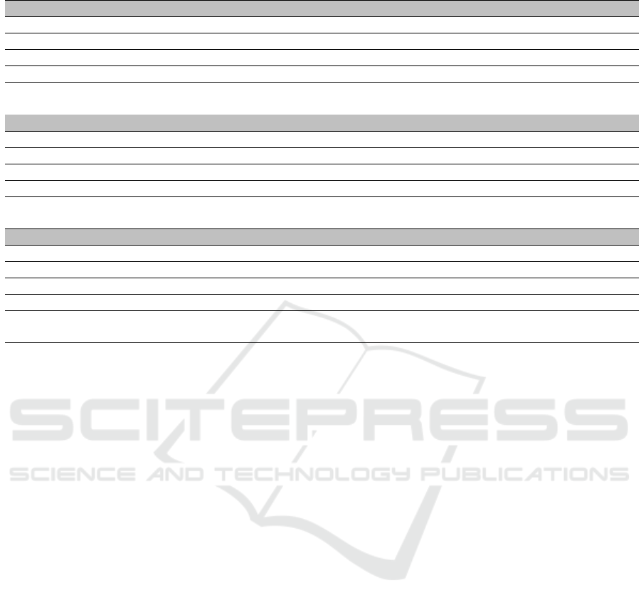
Table 13: Evaluation metrics in regard to perturbation assessment.
Random Forest Classifier
Dataset Accuracy Precision ‘too early’ Precision ‘on time’ Precision ‘too late’
Full test data set 73.43% 58.30% 78.22% 88.78%
Only unreliable input cases 49.90% 46.27% 58.79% 49.56%
Only reliable input cases 76.34% 62.31% 79.27% 90.77%
All unreliable cases adjusted
to the correct prediction
78.95% 68.68% 81.25% 91.24%
Gradient Boosting Classifier
Dataset Accuracy Precision ‘too early’ Precision ‘on time’ Precision ‘too late’
Full test data set 75.19% 65.86% 75.88% 89.50%
Only unreliable input cases 55.95% 57.20% 55.41% 50.08%
Only reliable input cases 80.07% 72.32% 79.46% 93.59%
All unreliable cases adjusted
to the correct prediction
84.10% 84.06% 82.45% 94.38%
Adaptive Boosting Classifier
Dataset Accuracy Precision ‘too early’ Precision ‘on time’ Precision ‘too late’
Full test data set 71.46% 59.07% 72.30% 89.01%
Only unreliable input cases 53.22% 53.69% 51.88% 56.97%
Only reliable input cases 75.37% 66.22% 74.19% 91.59%
All unreliable cases adjusted
to the correct prediction
79.71% 83.10% 77.11% 92.51%
2.59 percentage points higher (5.52% − 2.93%) than
when the expert would look at the same amount of
randomly selected cases, which means that the accu-
racy gain when checking unreliable cases returned by
the perturbation approach is 88% (5.52% ÷ 2.93%)
greater than if the expert looked at the same number of
randomly selected cases to manually verify and cor-
rect predictions.
Considering the gradient boosting classifier, us-
ing the perturbation options described in Section 3
we found 13 315 unreliable input cases. Thus,
20.23% (13 315 ÷ 65 801) of all test cases were
marked as unreliable by the perturbation approach.
If a human expert conducted a closer examination
of all these unreliable cases then, under the assump-
tion that the expert is able to manually determine
the correct prediction for all these cases, the over-
all accuracy of the model would rise from 75.19% to
84.10% representing a potential improvement of 8.91
percentage points in accuracy that can be achieved
with the perturbation assessment. The maximum pos-
sible overall accuracy increase is 24.81 percentage
points (100% − 75.19%), if all 65 801 are checked
by a human expert who is able to correct the predic-
tion. Hence, if a human expert were to look at the
randomly drawn samples to manually verify and cor-
rect the predictions, the accuracy would rise on aver-
age by 5.02% (24.81% × 0.2023). Compared to this,
if the expert were to look at the unreliable cases re-
turned by the perturbation approach, we could poten-
tially achieve an increase in overall accuracy that is
3.89 percentage points higher (8.91% − 5.02%) than
when the expert would look at the same amount of
randomly selected cases, which means that the accu-
racy gain when checking unreliable cases returned by
the perturbation approach is 77% (8.91% ÷ 5.02%)
greater than if the expert looked at the same number of
randomly selected cases to manually verify and cor-
rect predictions.
Considering the adaptive boosting classifier, us-
ing the perturbation options described in Section 3
we found 11 600 unreliable input cases. Thus,
17.62% (11 600 ÷ 65 801) of all test cases were
marked as unreliable. If a human expert conducted
a closer examination of all these unreliable cases
then, under the assumption that the expert is able
to manually determine the correct prediction for all
these cases, the overall accuracy of the model would
rise from 71.46% to 79.71% representing a poten-
tial improvement of 8.25 percentage points in accu-
racy that can be achieved with the perturbation as-
sessment. The maximum possible overall accuracy
increase is 28.54 percentage points (100%−71.46%),
if all 65 801 are checked by a human expert who is
able to correct the prediction. Hence, if a human ex-
pert were to look at the randomly drawn samples to
manually verify and correct the predictions, the ac-
curacy would rise on average by 5.03% (28.54% ×
0.1762). Compared to this, if the expert were to look
at the unreliable cases returned by the perturbation ap-
proach, we could potentially achieve an increase in
overall accuracy that is 3.22 percentage points higher
Implementing the Perturbation Approach for Reliability Assessment: A Case Study in the Context of Flight Delay Prediction
83

(8.25% − 5.03%) than when the expert would look at
the same amount of randomly selected cases, which
means that the accuracy gain when checking unre-
liable cases returned by the perturbation approach
is 64% (8.25% ÷ 5.03%) greater than if the expert
looked at the same number of randomly selected cases
to manually verify and correct the predictions.
5 TOOL SUPPORT
In the initial perturbation approach, we implemented
any code components, which were necessary to per-
turb new input cases, besides the implementation of
the model-related parts. This was done without any
user interface and a lot of steps had to be repeated for
each assessment in different use cases. Therefore, we
decided to provide generic tool support which encap-
sulates all parts of the perturbation approach, that are
not specific to a given use case, like generic perturba-
tion options or the combinatorial logic used to form
the test cases.
5.1 Core Functionality
The user interface is organized into the six sec-
tions: Home, Data Understanding, Data Preprocess-
ing, Prediction Model, Modeling, and Deployment,
each of which offers different capabilities to the user.
The Home section is the starting point for reliability
assessment for a new use case. Any modeled infor-
mation is stored in a knowledge graph, thus the Home
section offers the possibility to create a new or se-
lect an existing knowledge graph from the configured
graph store. When a new knowledge graph is created,
the user must upload a JSON file containing metadata
about the features of the prediction model.
The Data Understanding section of the tool is in-
tended to collect any knowledge about the features
that may provide a starting point for perturbation.
Currently, we have implemented four different cate-
gories of information related to data understanding.
First, we are interested in the metadata of the fea-
tures, containing the name of the feature, scale of
measurement, and all allowed values for a feature.
The metadata must be provided for the tool in order to
work properly, so we decided to include this informa-
tion in the mandatory input JSON. Second, the real-
world volatility of a feature provides information on
whether the feature value could change shortly after it
is recorded, thus providing a good candidate for per-
turbation. For example, a sensor measuring the wind
speed might have yielded a different value if the mea-
surement would have been taken a few seconds before
or after the actual measurement. In this case, the user
has the possibility to indicate one of the three volatil-
ity levels—low volatility, medium volatility, or high
volatility—for each of the features. Third, a specific
domain or use case may have specific value restric-
tions that cannot occur for a case. For example, the
feature age cannot have a value under 18 because 18
is the minimum legal age to apply for a loan. The user
has the possibility to indicate case-specific value re-
strictions, which will later restrict the creation of per-
turbed test cases. Fourth, using sensors to measure a
feature value, it may occur that the sensor measures a
value that differs from the actual value within a given
sensor precision. For example, measuring the temper-
ature using a temperature sensor with a sensor preci-
sion of ±10% means that the real-world value may
differ 10% from the measured value. The user has the
possibility to indicate any known sensor precision for
the features. This list of information items related to
data understanding is not exhaustive and may be ex-
tended in the future.
The Data Preprocessing section of the tool is in-
tended to collect any knowledge on alterations that
were applied to the features to prepare the data for the
training of the prediction model. Currently, we have
implemented two different categories of data prepro-
cessing information. First, a user has the possibility to
document whether a feature was altered by the use of
binning and, second, how missing values for a feature
were addressed during data preprocessing. The list of
data preprocessing information described here is not
exhaustive and may be extended in the future.
The Prediction Model section of the tool is in-
tended to upload and choose the prediction model
which should be used to retrieve the predictions for
the perturbed test cases. The user must ensure that
the input features used to train the model are con-
sistent with the features which were specified in the
mandatory metadata JSON input file.
The Modeling section of the tool allows to choose
and customize perturbation options for features. First,
the user specifies which of the predefined perturba-
tion options may be used for each feature. For exam-
ple, a chosen option may be the step-wise perturba-
tion of a feature age, which would create perturbed
test cases by adding and subtracting a defined number
of years from the original value. Second, the user can
customize any chosen perturbation options. The cus-
tomization process includes the following three steps:
choice of information on which the perturbation op-
tion was based, specification of any possible parame-
ters of a perturbation option, and the specification of
the perturbation level of the respective perturbation
option. After every chosen perturbation option is cus-
ICEIS 2025 - 27th International Conference on Enterprise Information Systems
84

tomized, the user has the possibility to save the collec-
tion of chosen perturbation options to the knowledge
graph. A saved collection can be used in deployment
to load this set of options for a new input case. It is
possible to create multiple collections of perturbation
options for one prediction project.
The Deployment section of the tool allows to se-
lect a predefined collection of perturbation options
and apply these perturbation options to new input
cases, thus creating a perturbation assessment for the
respective input case. A user can select one of the
predefined collections of perturbation options from a
drop-down menu. The tool provides the possibility
to view all perturbation options that are included in
the chosen collection as well as to add additional or
to remove included perturbation options from the col-
lection before starting with the assessment of a new
case. Once the user has selected all perturbation op-
tions that should be used for the assessment, the new
input cases should be entered into the tool. A new
case can be entered either by entering a value for each
feature in the user interface, or by uploading a CSV
file that contains the feature values. All entered cases
are shown within a table in the user interface. The
user can click on one of the cases in the table and af-
ter providing a label for this case, the user can start
perturbing of the respective case. After the process-
ing of the perturbed test cases is finished, the result is
shown within a table in the user interface. The result
consists of the original input case, shown in the first
line of the table, and all perturbed test cases which
are created based on the chosen perturbation options.
Each perturbed test case in the result highlights all
perturbed values for the user. Besides the table that
includes all perturbed cases, the user also gets a table
where only those perturbed cases are shown that re-
ceived a changed prediction compared to the original
input case. Perturbed test cases with a changed pre-
diction are of interest for a domain expert to assess the
reliability of the original case’s prediction. The user
has the possibility to download all perturbed cases in
CSV format for further processing.
5.2 Architecture
We decided against building a heavyweight RESTful
implementation of the tool in favor of the lightweight
Python framework Streamlit
4
, which offers enough
flexibility to demonstrate the functionality, including
a simple graphical user interface. As database we
used the Fuseki
5
graph store, which saves any relia-
bility assessment information in the format proposed
4
https://streamlit.io/
5
https://jena.apache.org/documentation/fuseki2/
{
” W i n d D i r e c t i o n ” : {” l e v e l O f S c a l e ” : ” C a r d i n a l ” ,
” u n i q u e V a l u e s ” : [ ” 5 ” , ” 3 6 0 ” ] } ,
” W i n g l e t s ” : {” l e v e l O f S c a l e ” : ” No minal ” ,
” u n i q u e V a l u e s ” : [ ”Y” , ”N” ] } ,
” Runway ” : {” l e v e l O f S c a l e ” : ” O r d i n a l ” ,
” u n i q u e V a l u e s ” : [ ” 0 ” , ” 0 . 2 ” , ” 0 . 4 ” , ” 0 . 6 ” , ” 0 . 8 ” , ” 1 ” ] }
}
Listing 1: Example JSON definition of feature metadata
by Staudinger et al. (2024). In the root folder of
the tool a user can find the three main configuration
files config, sparql, and strings. The config file con-
tains configurable items, e.g., the link to the graph
store. The sparql file contains all SPARQL-queries
that are used to insert or retrieve information from the
graph store, so if any changes to the knowledge graph
schema are necessary, they can be made here. The
strings file contains any text that is shown within the
tool, thus enables easy textual changes or the provi-
sion of the tool in another language.
The tool uses two main inputs in order to assess
the reliability of individual predictions. The first in-
put is a JSON file describing the metadata of the fea-
tures of the prediction model. An illustrative exam-
ple of the structure of the JSON file is shown in List-
ing 1. Every feature is listed with its unique name
(e.g., Wind Direction), its scale of feature (levelOfS-
cale), which can either be Cardinal, Nominal, or Or-
dinal, and the unique values (uniqueValues) for each
feature. A cardinal feature should specify a mini-
mum (e.g., 5) and a maximum (e.g., 360) value that
is allowed for this feature. Nominal and ordinal fea-
tures should specify a list of all allowed feature values
whereby the list should be ordered for ordinal features
(e.g., “0”, “0.2”, “0.4”). The information, contained
in the JSON file, is the minimum information that is
required in order to perform the assessment.
The second input is an already trained prediction
model. Since the training of prediction models can
take hours, it is not possible to retrain a model ev-
ery time the tool is started. Therefore, we offer the
possibility to upload any pre-trained model that was
exported using the python library pickle
6
. Once up-
loaded, the user can choose which prediction model
should be used for a new input case.
The output of the tool is a collection of perturbed
test cases, which is presented in the user interface. A
user has the possibility to download the collection in
CSV format, where the first line represents the orig-
inal test case and all following rows represent per-
turbed test cases, including the respective prediction
6
https://docs.python.org/3/library/pickle.html
Implementing the Perturbation Approach for Reliability Assessment: A Case Study in the Context of Flight Delay Prediction
85

of the chosen prediction model.
In addition to the reliability assessment, which
consists of all perturbed test cases, the tool captures
the provenance of any used and modeled information
that was included in the assessment in a knowledge
graph, following the reference process described by
Staudinger et al. (2024). Once the assessment is done,
it is possible to recognize which information was the
reason for the chosen perturbation options and which
options were used within the specific perturbation as-
sessment. The source code of the prototype is avail-
able online
7
.
6 CONCLUSIONS
In this paper, we demonstrated how to conduct relia-
bility assessment for flight delay predictions using a
perturbation approach, including the required imple-
mentation steps. The real-world use case was inspired
by Bardach et al. (2020), from which we reused some
of the training data for the development of our own
prediction models. For implementing the perturbation
approach in this use case, we followed the reference
process proposed by Staudinger et al. (2024) and de-
scribed what information related to reliability assess-
ment was documented in the course of development
of the prediction model. This documented informa-
tion is the basis for using various perturbation options,
which serve to assess the reliability of predictions in
the test data set that was used for the evaluation of the
prediction model.
Future work may further investigate the impact
of different admissible ranges of the parameter val-
ues for the perturbation options on the performance of
reliability assessment. Furthermore, the perturbation
approach may be extended into multi-feature pertur-
bation, thus being able to detect potentially unreliable
input cases when only the combination of perturbed
features leads to a changed prediction.
REFERENCES
Bardach, M., Gringinger, E., Schrefl, M., and Schuetz, C. G.
(2020). Predicting flight delay risk using a random forest
classifier based on air traffic scenarios and environmental
conditions. In 2020 AIAA/IEEE 39th Digital Avionics
Systems Conference (DASC), pages 1–8. IEEE.
Bureau of Transportation Statistics (2024). Bureau of
Transportation Statistics. https://transtats.bts.gov/
DatabaseInfo.asp?QO VQ=EFD&DB URL=Z1qr VQ=
E&Z1qr Qr5p=N8vn6v10&f7owrp6 VQF=D, Accessed
on 29.10.2024.
7
https://doi.org/10.5281/zenodo.14721638
Carri
´
o, P., Pinto, M., Ecker, G. F., Sanz, F., and Pastor, M.
(2014). Applicability domain analysis (ADAN): A ro-
bust method for assessing the reliability of drug property
predictions. J. Chem. Inf. Model., 54(5):1500–1511.
Chen, T. Y., Kuo, F., Liu, H., Poon, P., Towey, D., Tse,
T. H., and Zhou, Z. Q. (2018). Metamorphic testing: A
review of challenges and opportunities. ACM Comput.
Surv., 51(1):4:1–4:27.
EUROCONTROL (2024). Network Manager Annual
Report 2023. https://www.eurocontrol.int/publication/
network-manager-annual-report-2023, Accessed on
16.10.2024.
Federal Aviation Administration (2024). Federal
Aviation Administration Aircraft Characteristics
Database. https://www.faa.gov/airports/engineering/
aircraft char database, Accessed on 30.10.2024.
Iowa State University (2024). Iowa environmen-
tal mesonet. https://mesonet.agron.iastate.edu/request/
download.phtml, Accessed on 22.10.2024.
Lor
¨
unser, T., Sch
¨
utz, C. G., and Gringinger, E. (2021).
Slotmachine - A privacy-preserving marketplace for slot
management. ERCIM News, 2021(126).
Pianosi, F., Beven, K. J., Freer, J., Hall, J. W., Rougier, J.,
Stephenson, D. B., and Wagener, T. (2016). Sensitivity
analysis of environmental models: A systematic review
with practical workflow. Environ. Model. Softw., 79:214–
232.
Siegel, E. (2013). Predictive analytics: The power to pre-
dict who will click, buy, lie, or die. John Wiley & Sons.
Staudinger, S., Schuetz, C. G., and Schrefl, M. (2024). A
reference process for assessing the reliability of predic-
tive analytics results. SN Comput. Sci., 5(5):563.
Wirth, R. and Hipp, J. (2000). CRISP-DM: Towards a Stan-
dard Process Model for Data Mining.
Yang, Y. and Chui, T. F. M. (2021). Reliability assess-
ment of machine learning models in hydrological pre-
dictions through metamorphic testing. Water Resources
Research, 57(9):e2020WR029471.
ICEIS 2025 - 27th International Conference on Enterprise Information Systems
86