Smoke Segmentation Improvement Based on Fast Segment Anything
Model with YOLOv11 for a Wildfire Monitoring System
Puchit Bunpleng
1 a
, Puthtipong Thunyatada
1 b
, Bhutharit Aksornsuwan
1 c
,
Kanokvate Tungpimolrut
2 d
and Ken T. Murata
3 e
1
Sirindhorn International Institute of Technology, Thammasat University, Pathum Thani, Thailand
2
NECTEC, National Science and Technology Development Agency, Pathum Thani, Thailand
3
National Institute of Information and Communications Technology, Tokyo, Japan
Keywords:
Wildfire, Smoke Segmentation, Machine Learning, YOLOv11, FastSAM, Gradient Boosting, Deep Learning.
Abstract:
Forests and wildlife are crucial parts of our ecosystem. Wildfires occurring in dry and hot regions represent
a significant threat to these areas, particularly in ASEAN countries during the dry season. While human
observers are often employed to detect wildfires, their scarcity and limited availability highlight the need for
automated solutions. This study explores the use of machine learning, specifically computer vision, to enhance
wildfire detection by segmenting smoke, an approach which potentially gives information regarding the size
and the direction of the spread of the smoke, aiding mitigation efforts. We extend prior work by proposing a
model to predict the errors and performance of segmentation masks without access to the ground truth, with
the aim of facilitating iterative self-improvement of segmentation models. The FireSpot dataset is used to
fine-tune a YOLOv11 model to predict bounding boxes of smoke successfully; subsequently, the outputs of
this model are used as a prompt to refine a FastSAM model designed to segment the image into a proposed
mask containing the smoke. The proposed mask and the corresponding original image are then used to train a
machine learning model where the targets are metrics regarding the error rates of the masks. The results show
that a gradient boosting model achieves good prediction performance in predicting some error metrics like the
IoU (denoted TPP in this paper) between the proposed and actual segmentation masks with an MSE of 0.03
and R
2
of 0.46, as well as the proportion of false positives over the union of the proposed and actual masks
(denoted FPP in our paper) with an MSE of 0.0002 and R
2
of 0.95, while a pre-trained deep learning model
fails to learn the distribution, achieving considerably lower performance for IoU with an MSE of 0.05 and R
2
of 0.06 and FPP with an MSE of 0.0002 and R
2
of -1.15. These findings open the way to future work where
the results of the error prediction model can be used as feedback to improve the prompts and hyperparameters
of the segmentation model.
1 INTRODUCTION
Forests and wildlife play a vital role in sustaining
ecosystems, providing essential resources such as
food, water, and air (Meena, 2021). However,
these natural resources are increasingly threatened by
disasters like wildfires (Gill et al., 2013). Wildfires
not only result in the loss of wildlife and destruction
of vegetation but also contribute to air pollution
a
https://orcid.org/0009-0005-7077-1024
b
https://orcid.org/0009-0004-4759-9863
c
https://orcid.org/0009-0005-4374-7918
d
https://orcid.org/0000-0001-8762-5967
e
https://orcid.org/0000-0002-4141-562X
through the release of smoke and dust particles
(Sukitpaneenit and Kim Oanh, 2014). Thus, it is
imperative to develop effective measures to protect
these environments.
Wildfires occur due to both natural and human-
induced factors (Chapin III et al., 2000). Traditional
methods to detect wildfire, such as watchtowers and
forest rangers, may be insufficient for early detection.
Recent advances in artificial intelligence (AI) could
mitigate the problem by enabling the development
of novel approaches to enhance wildfire detection
capabilities. AI-driven systems have the potential to
identify wildfires in their early stages, allowing for
timely alerts to relevant personnel and preventing the
fire from spreading (Barmpoutis et al., 2020).
Bunpleng, P., Thunyatada, P., Aksornsuwan, B., Tungpimolrut, K. and Murata, K. T.
Smoke Segmentation Improvement Based on Fast Segment Anything Model with YOLOv11 for a Wildfire Monitoring System.
DOI: 10.5220/0013299300003944
Paper published under CC license (CC BY-NC-ND 4.0)
In Proceedings of the 10th International Conference on Internet of Things, Big Data and Security (IoTBDS 2025), pages 129-140
ISBN: 978-989-758-750-4; ISSN: 2184-4976
Proceedings Copyright © 2025 by SCITEPRESS – Science and Technology Publications, Lda.
129

Wildfire smoke detection has been the subject
of various research efforts, utilizing both traditional
image processing and more recent deep learning
based methods. Traditional image segmentation
methods, such as edge detection and thresholding,
have been commonly applied for smoke detection.
For instance, Sobel and Canny edge detection
techniques have achieved high mean intersection over
union (mIoU) scores in wildfire smoke detection
(Chaturvedi et al., 2021). However, these methods
often fail when dealing with complex environments
such as smoke-filled or foggy conditions.
Recent studies have also focused on deep
learning-based segmentation methods to improve
smoke detection accuracy. The use of convolutional
neural networks (CNNs) has gained significant
attention due to their effectiveness in image
recognition tasks. One study proposed a CNN-based
framework that combines EfficientNet for smoke
detection and DeepLabv3+ for segmentation, which
achieved notable improvements in both accuracy and
reducing false alarm rates (Khan et al., 2021). This
approach was designed to handle both clear and
hazy environments, making it suitable for real-world
wildfire surveillance scenarios.
Additionally, another study introduced a method
that utilizes local extremal region segmentation
(MSER) for detecting smoke in video frames.
This technique efficiently identifies potential smoke
regions by selecting stable extremal regions in the
image and tracks these regions across frames for
continuous monitoring. The authors demonstrated
that their method effectively detects long-distance
wildfire smoke and is robust to camera shake caused
by strong winds, making it a reliable solution for real-
time monitoring (Zhou et al., 2016).
However, to our knowledge, no previous work has
proposed a model to predict accuracy or error metrics
such as IoU of the segmentation model in order to
iterate and optimize said model’s parameters.
Our study focuses on leveraging computer vision,
a branch of AI that enables machines to process
visual media such as images or videos (Voulodimos
et al., 2018). Specifically, we propose a system that
utilizes object detection and segmentation techniques
to identify wildfire smoke and assess the scale of
the fire and its spreading direction. Integrating
these techniques can improve the accuracy of smoke
detection and provide more precise information about
the fire’s extent.
For this purpose, we employ the FireSpot database
(Pornpholkullapat et al., 2023) developed through
collaboration among the National Electronics and
Computer Technology Center (NECTEC) and local
municipalities in Chiang Mai, Thailand (Pa Miang,
Nong Yaeng, and Choeng Doi). This dataset
comprises approximately 4,000 images captured
in controlled conditions, with both smoke and
non-smoke scenarios, enabling robust training and
evaluation of the proposed AI models.
The dataset development was one of the key
results of a collaborative research project among four
ASEAN countries (Thailand, Myanmar, Lao PDR,
and the Philippines) and Japan under the ASEAN
IVO framework to address common environmental
problems.
The rest of this paper is organized as follows.
Section 2 introduces the necessary background
concepts and models that have been employed
within this paper. Section 3 details our proposed
method, starting from the overall detection and
classification pipeline, and details each step from the
smoke detection, smoke segmentation, segmentation
model optimization, and mask error detection
model. Section 4 continues with the results of our
experiments outlined in Section 3 and the evaluation
thereof. Section 5 discusses the implications and
analysis of the results obtained, as well as possible
further applications. We conclude with Section 6
where we summarize our intentions and work done,
as well as avenues for future work.
2 BACKGROUND
This section provides the prerequisite concepts and
models that are used in this paper. Specifically, we
will discuss the YOLOv11 model (Jocher and Qiu,
2024), and FastSAM (Zhao et al., 2023) developed by
Ultralytics, pre-trained models, and gradient boosting
models.
2.1 Pre-Trained Models
The term “pre-trained” refers to machine learning
models that have already been trained on a large and
diverse dataset to perform specific tasks (Pan and
Yang, 2010). These models are typically available
for immediate use, allowing researchers to apply them
directly to new data. Furthermore, pre-trained models
can be fine-tuned using additional datasets to adapt to
specific requirements or to enhance performance for
particular tasks by, for example, appending several
trainable fully connected layers over the pre-trained
backbone. This approach can significantly reduce
both the computational cost and the time required
for training models from scratch (Pan and Yang,
2010). Some examples of commonly used pre-trained
IoTBDS 2025 - 10th International Conference on Internet of Things, Big Data and Security
130

models in applications involving image processing
include ResNet (He et al., 2015) and EfficientNet (Tan
and Le, 2019).
2.2 YOLOv11
YOLO (You Only Look Once) version 11 or
YOLOv11 (Jocher and Qiu, 2024) is the latest
iteration in the YOLO series of pre-trained models for
object detection developed by Ultralytics (Redmon
et al., 2016). YOLOv11 specializes in real-time
object detection and classification tasks, where it is
capable of quickly identifying and classifying objects
in images or videos. The model works by drawing
bounding boxes around detected objects, providing a
clear visual representation of each object’s location.
YOLOv11 has been optimized for both speed and
accuracy, making it highly efficient for deployment
in a variety of applications, in our case, in a
remote observation tower over a forest. Additionally,
the model can be fine-tuned on custom datasets to
improve its accuracy for specific use cases (Jocher
and Qiu, 2024).
2.3 FastSAM
Fast segment anything model or FastSAM is
another state-of-the-art pre-trained model developed
by Ultralytics (Zhao et al., 2023). FastSAM is capable
of high-performance image segmentation and is
optimized to be fast and lightweight, allowing usage
in real-time environments like a forest watchtower.
This means that FastSAM not only detects objects but
also generates mask images that precisely outline the
object’s shape. This capability is particularly useful
in applications that require detailed object boundaries,
such as identifying the direction of a smoke plume.
FastSAM has two branches: a detection branch
that outputs categories and bounding boxes, and
a segmentation branch that generates k prototypes
(default 32) and mask coefficients, which operate
in parallel. The segmentation branch uses a
high-resolution feature map to preserve spatial and
semantic details. This map undergoes convolution,
upscaling, and further convolution to produce
segmentation masks. Mask coefficients, ranging from
−1 to 1, are multiplied with the prototypes and
summed to yield the final segmentation output.
2.4 Gradient Boosting
Gradient boosting is a machine learning technique
used for both classification and regression tasks. It
works by building a series of small decision trees
with a small number of splits, where each successive
tree is trained on and incrementally corrects the errors
made by the previous one. Each iteration places more
emphasis on the observations that previous models
misclassified (Natekin and Knoll, 2013). Gradient
boosting models are highly accurate and resistant
to overfitting, and are capable of handling data
imbalance well due to their nature as an ensemble of
decision trees. Popular implementations of Gradient
Boosting include XGBoost (Chen and Guestrin,
2016), LightGBM (Ke et al., 2017), and CatBoost
(Dorogush et al., 2018), each offering optimized
versions of this algorithm. It is highly popular and
often viewed as the default model to use in handling
tabular data, especially in classification tasks.
3 PROPOSED METHOD
The proposed method follows a multi-step pipeline
for smoke detection and segmentation, illustrated in
Figure 1. Initially, we used the YOLOv11 model,
which detects smoke in the images and generates
bounding boxes. These bounding boxes are then
used as input to the FastSAM model, a pre-trained
segmentation model which supports prompting (that
is, additional input like text or positive points that
will provide hints as to the correct segmentation).
A bounding box is an example of a prompt which
the model uses to enhance segmentation capability.
Finally, the segmentation results are evaluated using
an error prediction model that estimates the accuracy
of the generated masks. We speculate that the
results of the final error prediction model can be used
to further adjust the prompts and hyperparameters
of the FastSAM model, hence iteratively improving
segmentation performance.
3.1 Smoke Detection
For smoke detection, we used the YOLO11m model.
The model was pre-trained with the COCO (Common
Objects in Context) dataset, but to adapt it to our
specific task, we fine-tuned it using a subset of the
FireSpot dataset, which contains approximately 800
images of smoke in various environments. The
dataset was split into 70% for training, 15% for
validation, and 15% for testing. The input was resized
to 640 pixels in both width and height before feeding
to the model. The model was trained with 40 epochs,
a batch size of 16 samples, and an adaptive moment
estimation with weight decay optimizer (AdamW).
The training yielded a model that could reliably
detect wildfire smoke. After fine-tuning, we obtained
Smoke Segmentation Improvement Based on Fast Segment Anything Model with YOLOv11 for a Wildfire Monitoring System
131

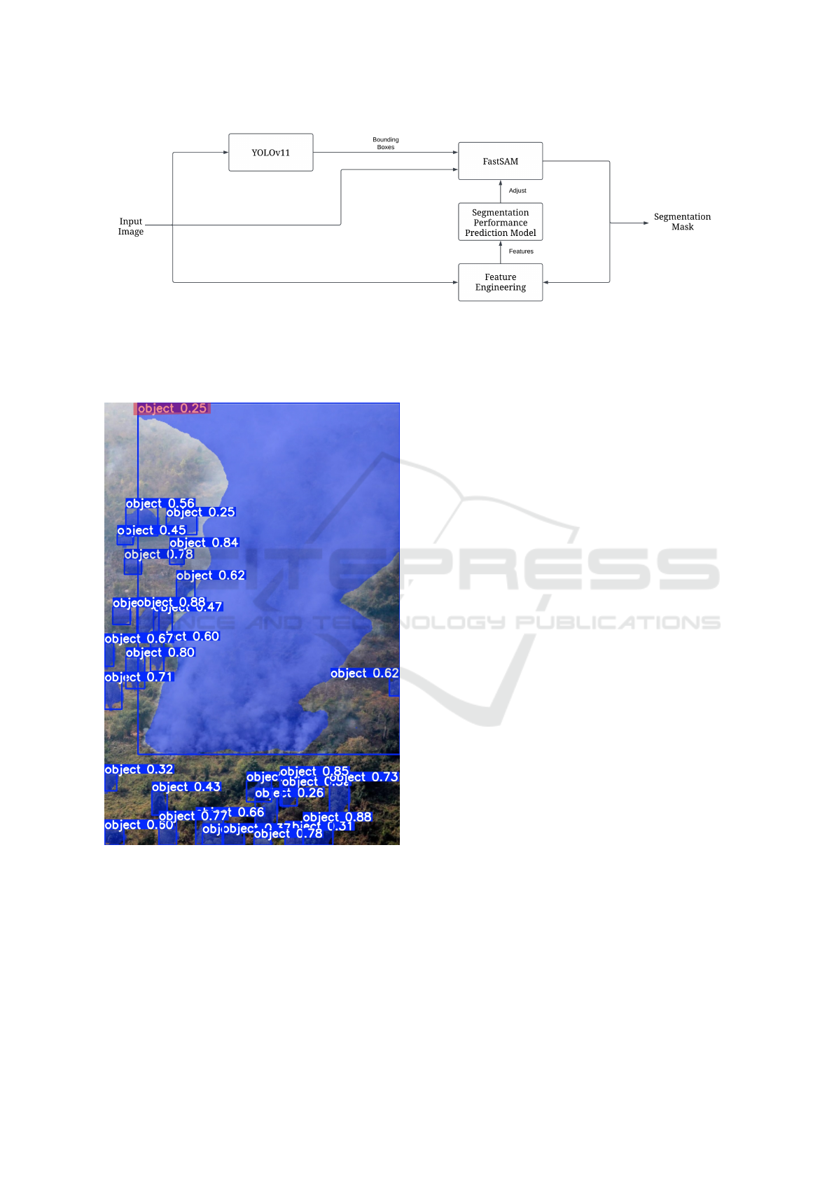
Figure 1: Overall process of the proposed method.
accurate bounding boxes that marked the locations of
the detected smoke. These bounding boxes were then
used as inputs for the subsequent segmentation model.
Figure 2: Visualization of the process behind FastSAM.
Each detected object within the images is highlighted
with a blue color and a bounding box. Each box has
its corresponding confidence score. The target object’s
confidence score is marked in red.
3.2 Smoke Segmentation
To segment the detected smoke areas, we employed
the FastSAM model, specifically the FastSAM-x
variant, which is the largest model and is designed
to segment objects using various prompt types.
Our model starts with a detection phase where an
object is detected if its confidence score exceeds a
threshold α. For smoke detection, we set α = 0.005,
which was informed by balancing precision and
recall to optimize overall performance. Preliminary
experiments demonstrated that as α increased, there
was a steady decline in precision, recall, F1 score,
accuracy, and IoU values. As for why setting α
value close to 0 helps improve performance, we
have to look at how FastSAM detects objects. To
find the reason behind this, we tried to visualize the
process behind FastSAM. We found that FastSAM
gave confidence values to every detected object in the
image, as shown in Figure 2. This value indicates
how confident the model recognizes each object in the
picture. As shown in Figure 2, the confidence value
of the smoke, which is our target object, is extremely
low, i.e., around 0.1 - 0.3. Setting the α to a high value
will reject the smoke and thus reduce the performance
of the proposed scheme. With this result, we can
conclude that an α value of 0 might be optimal but it
resulted in selecting all or sometimes random objects
instead of the smoke. After analyzing this behavior,
an α value of 0.005 was chosen as it provided
the best balance between precision and recall while
maintaining robust segmentation performance. This
is illustrated in Figure 3.
FastSAM supports multiple types of input
prompts, including bounding boxes, points, text, and
their combinations. We combine the prompts to tell
the FastSAM model what and where to detect the
objects it has found in from the detection phase, in this
case, the bounding boxes of the forest fire smoke and
text indicating it is looking for forest fire smoke. The
process of bounding box prediction and segmentation
is visualized in Figure 4.
IoTBDS 2025 - 10th International Conference on Internet of Things, Big Data and Security
132

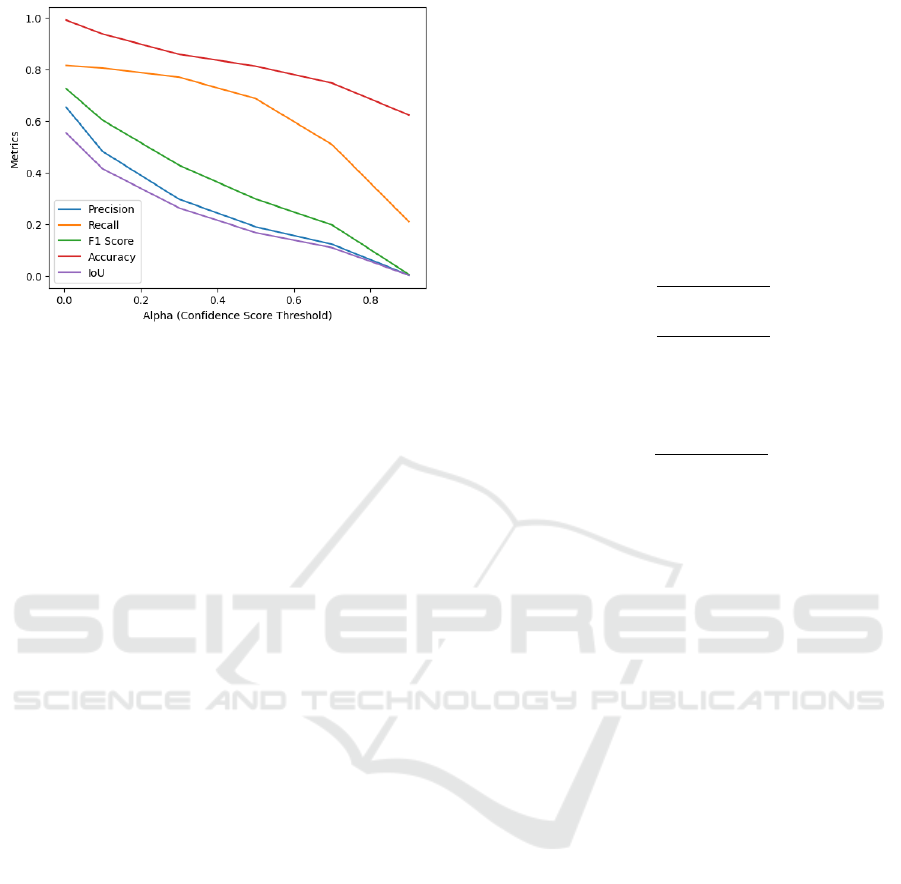
Figure 3: Performance metrics (precision, recall, F1 score,
accuracy, and IoU) as a function of α in FastSAM. The
chosen value of α = 0.005 achieves the best balance
between metrics.
3.3 FastSAM Model Optimization
Following segmentation, we implemented a scheme
to estimate the accuracy of the segmentation masks
generated by FastSAM in order to allow for the
optimization of the FastSAM model. Specifically,
we calculate the intersection over union (IoU) metric,
which measures the overlap between the predicted
segmentation mask and the ground truth mask. The
model considers a segmentation to be correct if the
IoU exceeds a threshold of 0.3. Segmentation masks
with IoU below 0.3 are considered incorrect, as
empirical observation during experimentation showed
that below this threshold the segmentation mask
was likely completely incorrect. To evaluate the
performance of the entire pipeline, we systematically
tested all combinations of prompts of the FastSAM
model. We found that the best result came from
using only the bounding boxes generated by the
YOLOv11 model as prompts. Other combinations,
such as adding point or text prompts, led to
decreased performance in segmentation accuracy.
With this, we obtained the currently optimal prompt
and hyperparameters to obtain the best possible
segmentation masks for our model. Hence, we
optimized the segmentation model for our final
component: a machine learning model which predicts
the various errors between the proposed segmentation
mask by FastSAM and the actual ground truth mask.
3.4 Segmentation Performance
Prediction Model
The proposed segmentation performance prediction
system is designed to estimate the accuracy of
the segmentation masks generated by the FastSAM
model from the previous section without access to the
ground truth mask. The system utilizes two primary
inputs: original images and their corresponding
proposed segmentation masks. Each mask is binary,
where pixels identified as smoke are marked as 1,
while the background is marked as 0. The objective
is to accurately predict three new values: True
Positive Proportion (TPP), False Negative Proportion
(FNP), and False Positive Proportion (FPP), which are
defined as follows:
TPP =
TP
TP + FP + FN
,
FNP =
FN
TP + FP + FN
,
and
FPP =
FP
TP + FP + FN
,
where TP (True Positive) represents the number
of pixels correctly identified as smoke in both the
predicted and ground truth masks, FP (False Positive)
represents the number of pixels identified as smoke in
the predicted mask but not in the ground truth mask,
and FN (False Negative) represents the number of
pixels identified as smoke in the ground truth mask
but missed in the predicted mask.
Note that the TPP is equivalent to the IoU
of the two masks. By normalizing these counts
relative to the union of the predicted and ground
truth masks, these metrics compensate for variations
in image dimensions and smoke coverage. This
method captures the impact of false negatives and
false positives in relation to the total area being
analyzed, making it more convenient to work with
than the raw pixel counts. This information can be
used to iteratively improve the pipeline by analyzing
the predicted proportions and adjusting prompts or
hyperparameters to enhance segmentation accuracy,
thereby optimizing the overall performance of the
segmentation pipeline.
To isolate the regions of the image relevant to
our regression task, we apply a masking algorithm
using the original image and its segmentation mask.
Let I denote the original image and M the binary
segmentation mask. The masking operation is defined
as:
D
i, j
=
(
I
i, j
if M
i, j
= 1,
0, if M
i, j
= 0.
(1)
Here, D represents the resulting masked image,
where (i, j) are the pixel coordinates. This step
filters out irrelevant background regions by retaining
Smoke Segmentation Improvement Based on Fast Segment Anything Model with YOLOv11 for a Wildfire Monitoring System
133

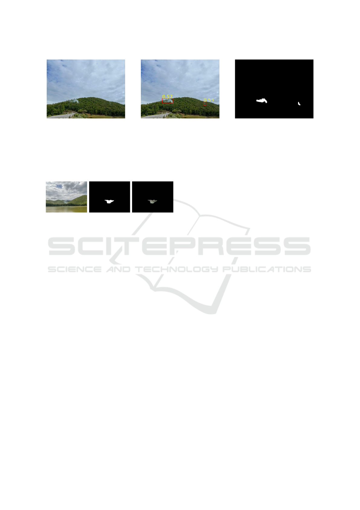
Figure 4: Original image (left), bounding boxes prediction on the original image predicted by the YOLOv11 model (center),
and segmentation masks predicted by the FastSAM model based on the bounding boxes from the center image (right).
only the pixels within the segmented area, while
setting the background to black (zero intensity). The
result is an image that focuses the analysis solely
on the regions identified as potential smoke. This
subtraction algorithm is illustrated in Figure 5.
Figure 5: Original image (left), segmentation masks of the
image predicted by FastSAM (center), and the resulting
image after application of the subtraction algorithm (right).
3.4.1 Feature Extraction
Once the background has been filtered, a set of
features from D that aim to differentiate smoke from
other natural elements such as trees and clouds are
extracted. The feature extraction process includes:
1. Color Histograms: Histograms are computed for
the RGB, HSV, and LAB color spaces to capture
the color distribution within the region of interest
(Swain and Ballard, 1991). These color spaces
are chosen because they provide complementary
representations of color information: RGB
captures raw color intensities, HSV separates
chromatic information from brightness, and
LAB approximates human perception of color
differences. Smoke regions often exhibit unique
color distributions characterized by muted tones
such as white, gray, or pale blue, which
contrast with the vivid greens of vegetation or
the bright blues of the sky. By quantifying
these differences, color histograms may be able
to distinguish smoke from natural elements,
improving detection.
2. Color Moments: We compute the mean, standard
deviation, and skewness for each channel of
the RGB, HSV, and LAB color spaces. These
moments provide statistical summaries of color
intensity distributions. The mean captures the
overall brightness and color tone, the standard
deviation reflects color variability, and skewness
identifies asymmetries in the distribution. These
metrics are particularly useful for identifying
smoke, which tends to have less variability and
more uniform tones compared to natural elements
like trees, which we hypothesize exhibit higher
color variability due to shadows and highlights
(Stricker and Orengo, 1995).
3. Edge Features: Edge density is computed using
the Canny edge detection algorithm (Canny,
1986). Smoke regions are often characterized
by a lack of sharp boundaries due to their
diffuse and amorphous nature, resulting in a
lower density of detected edges. In contrast,
tree canopies and other natural objects typically
exhibit well-defined, sharp edges. By capturing
this distinction, edge features play a crucial role in
differentiating smoke from other elements in the
scene. This makes edge analysis a key component
in reducing false positives during detection.
4. Texture Analysis Using GLCM: Texture
patterns are analyzed using the gray-level co-
occurrence matrix (GLCM), which extracts
features such as contrast, energy, and
homogeneity (Haralick et al., 1973). Smoke
often appears as a homogeneous or low-contrast
texture compared to the heterogeneous and high-
contrast textures of tree canopies or other natural
elements. For instance, the homogeneity metric
captures the smoothness of smoke regions, while
the contrast metric highlights the absence of
sharp intensity variations usually seen in textured
objects.
5. Color Coverage: To estimate the proportion of
grayscale tones indicative of smoke, we measure
the percentage of pixels that fall within a specific
range of gray values. Smoke typically exhibits
a high concentration of such tones, which is less
common in natural elements like trees or the sky.
This feature quantifies the prevalence of these
IoTBDS 2025 - 10th International Conference on Internet of Things, Big Data and Security
134

tones, providing another factor that enhances the
model’s ability to identify smoke regions.
The extracted feature vectors are then concatenated
in order to make them compatible with the regression
model input format.
3.5 Gradient Boosting Models
To predict the segmentation error metrics (FNP, TPP,
and FPP), we employ a set of gradient boosting
models. We utilize a multi-output regression
approach, where three separate gradient boosting
models are trained, one for each target metric.
Specifically, we compare multiple gradient boosting
algorithms, including Scikit-learn’s internal gradient
boosting regressor model (Pedregosa et al., 2018),
LightGBM (Ke et al., 2017), and XGBoost (Chen and
Guestrin, 2016). This is because our dataset shows
characteristics of imbalance, where most pictures tend
to cluster around the mean of the target metrics,
with a smaller, non-outlier subset deviating from that
mean. A model may be able to achieve low MSE
loss by predicting around the mean while ignoring the
deviating samples. We hypothesize gradient boosting
is capable of compensating for the imbalance in data.
The models use an 80:20 train-test split and are
evaluated using the mean squared error (MSE) and
the coefficient of determination (R
2
) on the validation
set.
3.5.1 Pretrained Deep Learning Models
To contrast with the above approach, we also
experiment with three pre-trained deep learning
models: ResNet18, ResNet50 (He et al., 2015),
and EfficientNet-B2 (Tan and Le, 2019), to predict
segmentation error metrics (FPP, TPP, and FNP).
These models are fine-tuned for the regression
task, using their backbone feature extractors, with
additional fully connected layers for prediction. The
output layer applies a sigmoid activation to constrain
predictions between [0, 1], since our targets are rates,
not counts.
For preprocessing, images and corresponding
masks are resized to 224 × 224 pixels after
concatenation of the image and mask together side-
by-side. The dataset is split 80:20 into training and
validation sets. We train for 10 epochs each using
MSE loss and a learning rate of 0.0001. The models
are evaluated using MSE and R
2
score. These deep
learning models’ performances are compared against
gradient boosting models in the next section.
4 RESULT AND EVALUATION
This section describes a detailed analysis of the
performance of our proposed method, including
fine-tuning results from YOLOv11, segmentation
performance using FastSAM, and comparisons
between gradient boosting and deep learning
models. Each component is evaluated across key
metrics to measure its effectiveness, accuracy, and
generalization capabilities.
4.1 YOLOv11 Fine-Tuning Results
We fine-tuned the YOLOv11-m model using the
FireSpot dataset, of which the subset we utilized
consists of approximately 800 images of smoke.
We observed consistent improvement across key
evaluation metrics over the 40 epochs of training. By
the final epoch, the model achieved a precision of 0.70
and recall of 0.72 on the validation set, with mean
average precision (mAP) scores of 0.74 at IoU 0.5 and
0.44 across IoU thresholds ranging from 0.5 to 0.95.
The box and objectiveness losses, for both training
and validation sets, also steadily decreased across the
40 epochs. These results, shown in Figure 6, suggest
that the model has learned to correctly identify the
location of the bounding boxes, which was visually
confirmed upon the plotting of the bounding boxes on
the images.
4.2 FastSAM Segmentation Results
In our experiments, we aimed to optimize the
parameters for the FastSAM model to identify the
most effective configuration for returning accurate
segmentation masks. We explored all combinations
of the following inputs: bounding box (bbox)
predictions from the YOLO model, text prompts fed
into the CLIP encoder, and labeled points classified as
positive or negative. Our findings showed that using
points alone resulted in only marginal segmentation
performance, with correct segmentation occurring
infrequently. Incorporating text prompts led to
moderate improvements, but the most significant
gains were achieved when using the bbox input.
Additionally, based on the metrics shown in
Figure 3, we discovered that lowering the confidence
threshold for segmentation improved the model’s
performance, as the model’s performance peaks when
the value of α approaches 0. On the other hand,
the performance slowly drops as the value of α
increases. This adjustment allowed the model to
accept bounding boxes with lower confidence scores,
thereby increasing the likelihood of capturing relevant
Smoke Segmentation Improvement Based on Fast Segment Anything Model with YOLOv11 for a Wildfire Monitoring System
135

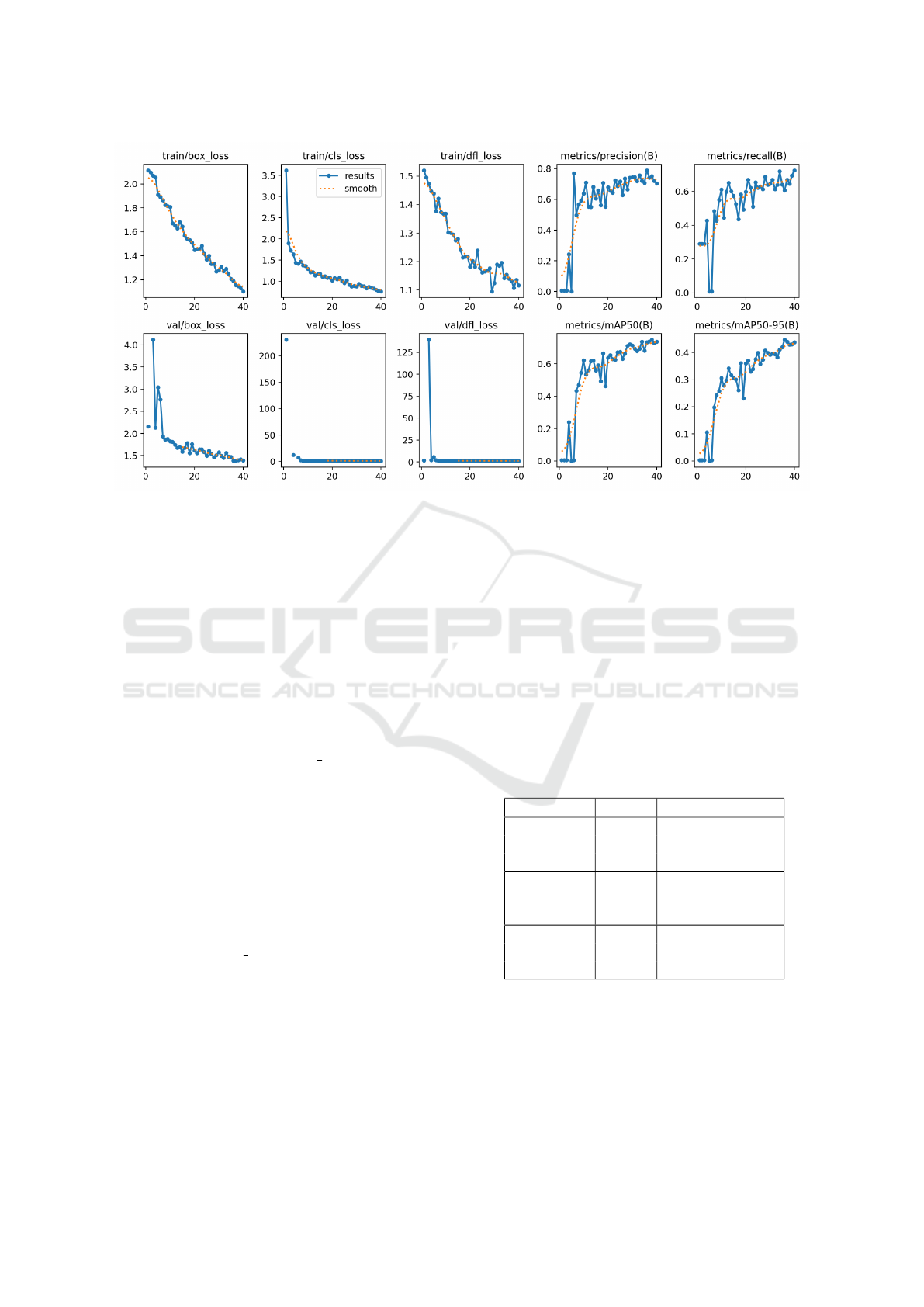
Figure 6: Training metrics of the YOLOv11 fine-tuning over 40 epochs.
regions and improving overall segmentation accuracy.
In the end, we found a confidence threshold of 0.005
was optimal.
4.3 Gradient Boosting Model Results
We used three gradient boosting models: XGBoost,
LightGBM, and Scikit-learn’s internal model, to
predict the error metrics based on features extracted
from segmented regions. The dataset consisted of
189 images, split into 80% training (151 samples)
and 20% testing (38 samples). Models were trained
using hyperparameters (n estimators=1000,
learning rate=0.05, max depth=6) without
additional tuning.
The chosen hyperparameter values were based on
experimentation across a wide range of values, during
which the models consistently demonstrated strong
performance despite several parameter changes. The
chosen settings provided good predictive accuracy
at relatively low computational cost, due to the
discovery that the models are not highly sensitive
to hyperparameter adjustments, meaning for example
a small value of n estimators could be chosen
without negative impact.
The Gradient Boosting models achieved the best
balance of performance and generalization compared
to the deep learning model. The results are shown in
Table 1. All three models did the best at predicting
TPP and FPP, where the MSE of the FPP for all three
models was consistently near zero, and the R
2
over
0.9 except for LightGBM, the weakest performer. The
same pattern is true in the TPP where the MSE tended
around 0.03 for all models and the R
2
all at around
0.45, indicating a strong generalization performance.
However, the worst performance these models had
was at predicting FNP: while the MSE was low at
around 0.05 for all models, the R
2
statistic is quite
low. The FNP is the proportion of the ground truth
not included in the proposed mask. As such, since
our preprocessing scheme involves retaining only the
proportion of the image in the proposed mask, it is
possible the relevant information to predict FNP was
not retained.
Table 1: Mean Squared Error (MSE) and R
2
scores for
different gradient boosting models predicting segmentation
error metrics.
Model Target MSE R
2
Scikit-learn
FNP 0.0523 -0.0404
TPP 0.0335 0.4164
FPP 0.0002 0.9604
LightGBM
FNP 0.0563 -0.1194
TPP 0.0315 0.4510
FPP 0.0010 0.7916
XGBoost
FNP 0.0567 -0.1285
TPP 0.0336 0.4607
FPP 0.0002 0.9404
4.4 Deep Learning Model Results
The training curves of ResNet50, as shown in Figure
7, ResNet18, and EfficientNet-B2, initialized with
standard parameters, exhibit similar trends over the
course of 10 epochs. Each model was trained on a
IoTBDS 2025 - 10th International Conference on Internet of Things, Big Data and Security
136

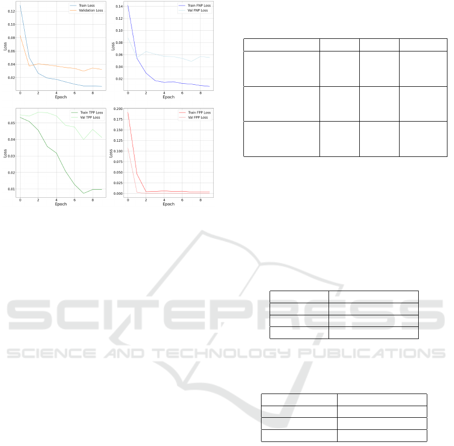
Figure 7: Average train and validation losses of the
ResNet50 model across 10 epochs (top left). The training
and validation loss curves for the FNP metric (top right).
The training and validation loss curves for the TPP metric
(bottom left). The training and validation loss curves for
the FPP metric (bottom right). The shape of these curves
is roughly representative of the loss curves of deep learning
models in this task in general.
dataset of 189 images, split 80:20 into training and
validation sets. The loss metrics, including training
and validation MSE, show a moderate decrease
during the first 1-2 epochs, followed by a plateau in
the later stages. This plateau occurred only in the
validation loss while the training loss still decreased,
indicating some degree of overfitting. Despite some
minor differences in early learning speeds, all models
have validation curves that are flat and do not
decrease like the training curves, indicating a failure
to generalize. The exception is the FPR loss, which
converges quickly to zero: this is because most values
in that metric are clustered around zero, the model
could simply predict values near zero to get a low
loss, meaning this doesn’t necessarily indicate true
learning by the model.
In Table 2, we also present the MSE and R
2
scores
for the deep learning models, which will be discussed
in the next section.
4.5 Inference Latency
This subsection provides an in-depth evaluation of
the inference latency for each model under controlled
conditions. Latency measurements were measured
by executing the prediction function seven times,
with 1000 iterations each to capture a robust average.
For the gradient boosting models, the tests utilized
Table 2: Mean Squared Error (MSE) and R
2
scores for
different deep learning models predicting segmentation
error metrics.
Model Target MSE R
2
ResNet50
FNP 0.0565 -0.0654
TPP 0.0462 0.0659
FPP 0.0002 -1.1521
ResNet18
FNP 0.0519 0.0622
TPP 0.0430 0.1278
FPP 0.0003 -4.1705
EfficientNet-B2
FNP 0.0502 0.0475
TPP 0.0439 0.0996
FPP 0.0007 -11.0456
the native CPU environment available in Google
Colab, and the resulting latency metrics are detailed
in Table 3. In contrast, the deep learning models
were evaluated on a more powerful computing setup,
specifically the T4 GPU provided by Google Colab,
with the corresponding latency results presented in
Table 4.
Table 3: Inference latency of gradient boosting models
predicting segmentation error metrics with Google Colab
CPU.
Model Inference Latency
Scikit-learn 4.97ms ± 429µs
LightGBM 8.36ms ± 468 µs
XGBoost 3.78ms ± 579 µs
Table 4: Inference latency of deep learning models
predicting segmentation error metrics with Google Colab
T4 GPU.
Model Inference Latency
ResNet18 35.1ms ± 850 µs
ResNet50 109ms ± 101 µs
EfficientNet-B2 67.3 ms ± 141 µs
5 DISCUSSION
The YOLO bounding box predictions performed
nearly optimally, accurately localizing objects in most
cases, with a very high IoU of over 0.99 when
tested on unseen data except for some outliers. The
FastSAM segmentation was also effective, with the
majority of segmentations aligning well with the
ground truth even without fine-tuning, due to the
optimizations in the hyperparameters and prompts we
performed. However, a few outliers were observed
where the model occasionally predicted the wrong
object, such as segmenting an entire mountain as
the target object. Furthermore, some masks were
Smoke Segmentation Improvement Based on Fast Segment Anything Model with YOLOv11 for a Wildfire Monitoring System
137

too small to cover the whole smoke, which will be
discussed later. Despite these errors, this section of
the pipeline is largely polished and functions reliably
as a preprocessing layer for our segmentation error
prediction model.
The results indicate that while the gradient
boosting models are generally effective at predicting
TPP, accurately predicting the FNP metric remains
challenging. This difficulty is likely due to the
subtraction process applied during feature extraction
of the gradient boosting model, where non-mask
regions of the image were removed. If smoke
was present but missed by the segmentation mask
(i.e., a false negative), these regions would also
be excluded, complicating the model’s ability to
predict FNP accurately. Similarly, the deep learning
models also face the same difficulties, having the
same low FNP and R
2
metrics (near zero, indicating
low loss but poor correlation), despite the fact that
the preprocessing process for these models simply
involves concatenation and resizing, not subtraction.
The failure of deep learning models to predict FNP
is possibly precisely because they have access to the
whole image, meaning most of the input is irrelevant
to the task at hand, preventing them from isolating
the features most important to isolating FNP, unlike
the gradient boosting models where the subtraction
algorithm eliminates the non-mask background.
This shortcoming is especially evident when
comparing the performance of gradient boosting
and deep learning models in terms of the TPP. At
first glance, it appears the gradient boosting models
slightly outperform the deep learning models by
achieving an MSE of around 0.03 as opposed to 0.04
for the deep learning models. However, we observe
that the gradient boosting models have a consistently
high R
2
value of nearly 0.5 while the deep learning
models have an R
2
of less than 0.1. Observing
the relationship between predicted and actual values
(see Figure 8) shows the reason why: deep learning
models do not actually learn the distribution of the
answers and generalize, but rather tend to predict in
a very narrow range of values which are commonly
observed. This strategy does indeed minimize MSE
loss but does not capture the full range of the data
due to an imbalanced dataset. However, the gradient
boosting models, while not perfect, show the ability
to generalize and predict a range of values across the
distribution.
For the FPP, both deep learning and gradient
boosting models have a practically nonexistent MSE.
This is because nearly all the FPP values are clustered
at near zero, which we will discuss promptly.
However, we also observe that the R
2
of gradient
boosting models with respect to the FPP is mostly
near 1, while the deep learning models have an R
2
that is extremely negative. This indicates the gradient
boosting models are far more capable of capturing the
true distribution of the FPP than the deep learning
models, which likely merely predicted low values
with no understanding of the underlying patterns.
We return to consider the distribution of the
outputs of the proposed segmentation masks given by
the YOLO segmentation model. As seen in Figure
8, the pattern is that the FPP is nearly nonexistent,
while the TPP and FNP are fairly distributed between
0 and 1. Given that the false positive (FP) count is
very low, while both the true positive (TP) and false
negative (FN) counts are nontrivial, this implies that
the predicted mask is smaller and likely contained
within the ground truth mask. The low FP count
indicates that the segmentation model accurately
identifies smoke pixels and does not mistake foliage
for smoke. However, the presence of nontrivial FN
values suggests that the model misses some regions
that are labeled as smoke in the ground truth, leading
to under-segmentation. This is confirmed by visual
inspection of some of the proposed masks (shown in
Figure 9), where it is very obvious that they are being
bounded by the bounding box prompts given by the
YOLO model. This suggests that the bounding boxes
are in fact, too small.
The deep learning models, such as ResNet50,
ResNet18, and EfficientNet-B2, demanded
significantly more GPU memory and computational
time for both training and inference. While these
models achieved low MSE values, their inflexibility in
handling varying input sizes and formats, along with
the tendency to overfit, limited their generalizability.
In contrast, gradient boosting models, while requiring
less computational power, offered a better balance
between MSE and R
2
scores, with more efficient
resource usage. This makes gradient boosting models
a more practical and adaptable choice, especially
for tasks with resource constraints or varying input
formats.
In summary, while gradient boosting models can
effectively predict certain segmentation error metrics,
addressing the issue of False Negatives requires
further work, possibly by incorporating additional
features or exploring improved preprocessing
methods in future work. Further research should be
done on more generalizable ways to extract features in
order to create models that can capture the full range
of real-life cases of forest fire sightings. Identifying
the most important features ranked by each gradient
boosting model can help us determine the most salient
part of the mask-subtracted image that differentiates
IoTBDS 2025 - 10th International Conference on Internet of Things, Big Data and Security
138

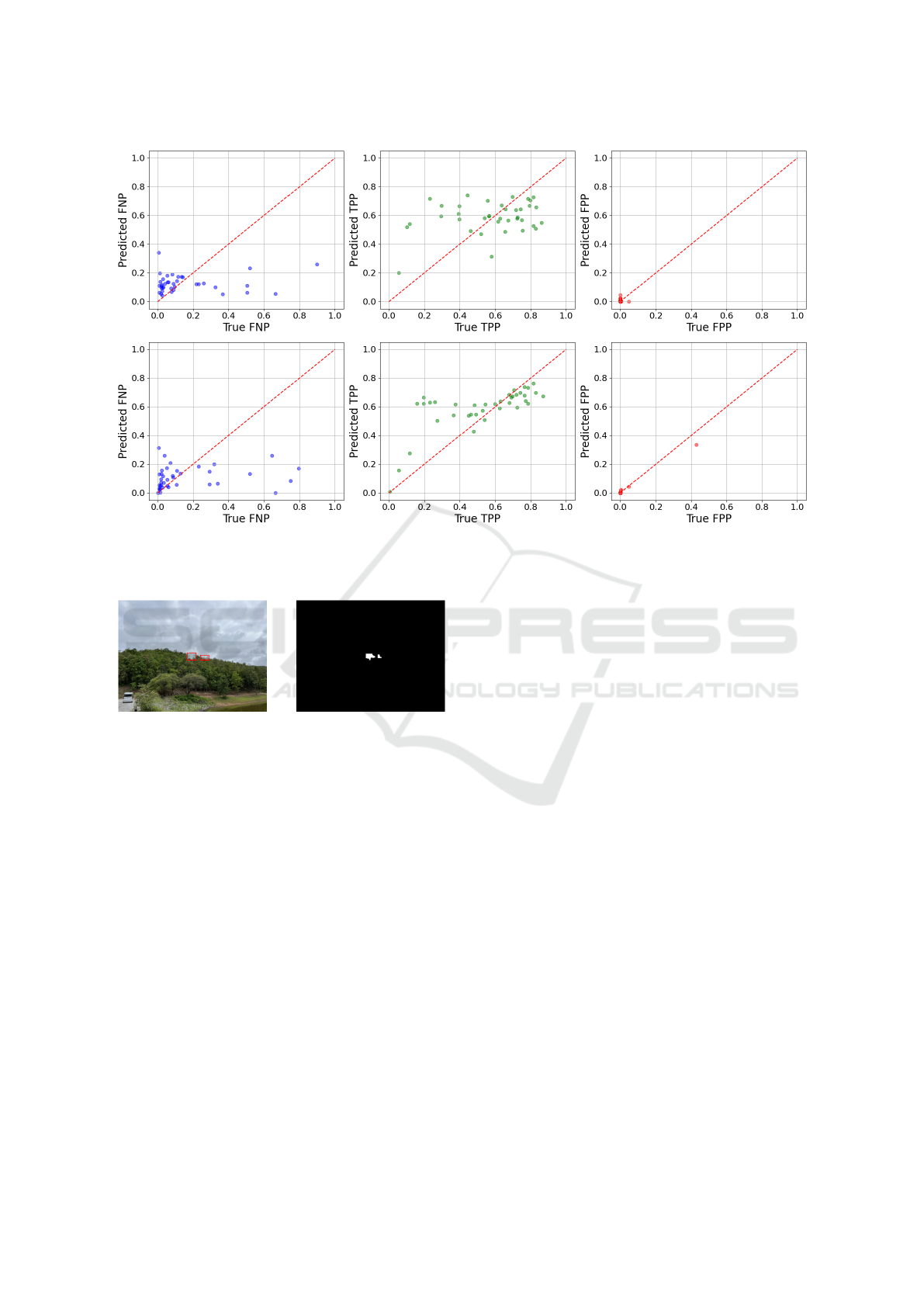
Figure 8: Predicted vs actual values plot for deep learning models for each of FNP, TPP, and FPP (top). The predicted vs
actual values plot for the gradient boosting models for each of FNP, TPP, and FPP (bottom). The gradient boosting models
show better performance across the entire distribution, particularly in the TPP and FPP metrics.
Figure 9: Original image (left). The proposed mask of the
left image is clearly bounded by the bounding box, thus
causing an underestimate compared to the true mask (right).
smoke and foliage. Additionally, constructing and
training segmentation error prediction models using
a balanced dataset may help mitigate model bias.
Another interesting path to explore is to utilize more
advanced promptable segmentation models which
may enhance segmentation accuracy, and to apply
this proposed method to segment things other than
smoke. Lastly, with further research, it might be
possible to utilize the proposed method to potentially
improve the model by determining the direction of
the plume, the size of the fire, or how long it has been
since the fire is up.
6 CONCLUSION
Wildfires are a major threat to forests and wildlife,
especially in ASEAN countries during the dry season.
One option to mitigate this problem is to employ
human observers. However, this might not be
feasible due to scarcity. Therefore, machine learning
can aid in addressing this challenge by applying
computer vision to detect wildfires for us. This study
extends the work on employing machine learning
algorithms to recognize and segment wildfire smoke
by introducing a model to predict the errors of the
segmentation mask, potentially opening up future
work regarding the iterative self-improvement of
wildfire segmentation models in response to new data.
By employing the FireSpot dataset to train
the YOLOv11 model to predict bounding boxes,
which are then used as prompts for the FastSAM
segmentation model, we find that our segmentation
model is already largely effective with a very high
IoU; however, a number of outliers and imperfections
remain in a minority of cases which could be
remedied for better performance. As a result, we
trained a series of machine learning models to predict
the errors of the segmentation masks and successfully
predicted the IoU (TPP) of the segmentation masks
using gradient boosting models with hand-crafted
features, though further work could be done in the
prediction of the FNP.
Experimentation was also done with pre-trained
deep learning models which found significantly
poorer generalization performance in all metrics, due
to data imbalance. Our method provides a promising
Smoke Segmentation Improvement Based on Fast Segment Anything Model with YOLOv11 for a Wildfire Monitoring System
139

avenue for future research regarding the possibility of
automated optimization of segmentation models.
ACKNOWLEDGEMENT
The ASEAN IVO project
(http://www.nict.go.jp/en/asean ivo/index.html),
titled ‘Visual IoT Network for Environmental
Protection and Disaster Prevention,’ was
involved in the production of the contents of
this work and financially supported by NICT
(http://www.nict.go.jp/en/index.html).
REFERENCES
Barmpoutis, P., Papaioannou, P., Dimitropoulos, K., and
Grammalidis, N. (2020). A review on early forest
fire detection systems using optical remote sensing.
Sensors, 20(22).
Canny, J. (1986). A computational approach to edge
detection. IEEE Transactions on pattern analysis and
machine intelligence, (6):679–698.
Chapin III, F. S., Zavaleta, E., Eviner, V., Naylor, R.,
Vitousek, P., Reynolds, H., Hooper, D., Lavorel, S.,
Sala, O., Hobbie, S., Mack, M., and Diaz, S. (2000).
Consequences of changing biodiversity. Nature,
405:234–42.
Chaturvedi, S., Khanna, P., and Ojha, A. (2021).
Comparative analysis of traditional and deep
learning techniques for industrial and wildfire smoke
segmentation. In 2021 Sixth International Conference
on Image Information Processing (ICIIP), volume 6,
pages 326–331.
Chen, T. and Guestrin, C. (2016). Xgboost: A scalable tree
boosting system. KDD ’16, page 785–794, New York,
NY, USA. Association for Computing Machinery.
Dorogush, A. V., Ershov, V., and Gulin, A. (2018).
Catboost: gradient boosting with categorical features
support.
Gill, A. M., Stephens, S. L., and Cary, G. J. (2013).
The worldwide “wildfire” problem. Ecological
Applications, 23(2):438–454.
Haralick, R. M., Shanmugam, K., and Dinstein, I. (1973).
Textural features for image classification. IEEE
Transactions on Systems, Man, and Cybernetics,
SMC-3(6):610–621.
He, K., Zhang, X., Ren, S., and Sun, J. (2015). Deep
residual learning for image recognition.
Jocher, G. and Qiu, J. (2024). Ultralytics yolo11.
Ke, G., Meng, Q., Finley, T., Wang, T., Chen, W., Ma, W.,
Ye, Q., and Liu, T.-Y. (2017). Lightgbm: A highly
efficient gradient boosting decision tree. Advances in
neural information processing systems, 30.
Khan, S., Muhammad, K., Hussain, T., Ser, J. D., Cuzzolin,
F., Bhattacharyya, S., Akhtar, Z., and de Albuquerque,
V. H. C. (2021). Deepsmoke: Deep learning model
for smoke detection and segmentation in outdoor
environments. Expert Systems with Applications,
182:115125.
Meena, D. (2021). A study on the importance of wildlife.
8.
Natekin, A. and Knoll, A. (2013). Gradient boosting
machines, a tutorial. Frontiers in Neurorobotics, 7.
Pan, S. J. and Yang, Q. (2010). A survey on transfer
learning. IEEE Transactions on Knowledge and Data
Engineering, 22(10):1345–1359.
Pedregosa, F., Varoquaux, G., Gramfort, A., Michel, V.,
Thirion, B., Grisel, O., Blondel, M., M
¨
uller, A.,
Nothman, J., Louppe, G., Prettenhofer, P., Weiss, R.,
Dubourg, V., Vanderplas, J., Passos, A., Cournapeau,
D., Brucher, M., Perrot, M., and
´
Edouard Duchesnay
(2018). Scikit-learn: Machine learning in python.
Pornpholkullapat, N., Phankrawee, W., Boondet, P.,
Thein, T. L. L., Siharath, P., Cruz, J. D., Marata,
K. T., Tungpimolrut, K., and Karnjana, J. (2023).
Firespot: A database for smoke detection in early-
stage wildfires. In 2023 18th International Joint
Symposium on Artificial Intelligence and Natural
Language Processing (iSAI-NLP), pages 1–6. IEEE.
Redmon, J., Divvala, S., Girshick, R., and Farhadi, A.
(2016). You only look once: Unified, real-time object
detection.
Stricker, M. A. and Orengo, M. (1995). Similarity of color
images. In Niblack, W. and Jain, R. C., editors,
Storage and Retrieval for Image and Video Databases
III, volume 2420, pages 381 – 392. International
Society for Optics and Photonics, SPIE.
Sukitpaneenit, M. and Kim Oanh, N. T. (2014). Satellite
monitoring for carbon monoxide and particulate
matter during forest fire episodes in northern
thailand. Environmental Monitoring and Assessment,
186(4):2495–2504.
Swain, M. J. and Ballard, D. H. (1991). Color indexing.
International Journal of Computer Vision, 7:11–32.
Tan, M. and Le, Q. V. (2019). Efficientnet: Rethinking
model scaling for convolutional neural networks.
ArXiv, abs/1905.11946.
Voulodimos, A., Doulamis, N., Doulamis, A., and
Protopapadakis, E. (2018). Deep learning for
computer vision: A brief review. Computational
Intelligence and Neuroscience, 2018(1):7068349.
Zhao, X., Ding, W., An, Y., Du, Y., Yu, T., Li, M., Tang, M.,
and Wang, J. (2023). Fast segment anything.
Zhou, Z., Shi, Y., Gao, Z., and Li, S. (2016). Wildfire smoke
detection based on local extremal region segmentation
and surveillance. Fire Safety Journal, 85:50–58.
IoTBDS 2025 - 10th International Conference on Internet of Things, Big Data and Security
140