A Computer Vision Approach to Fertilizer Detection and Classification
Jens Lippel
1 a
, Richard Bihlmeier
2 b
and Andr
´
e Stuhlsatz
1,2 c
1
Department of Mechanical and Process Engineering, University of Applied Sciences Duesseldorf, Germany
2
FMDauto - Institute for Product Development and Innovation, University of Applied Sciences Duesseldorf, Germany
Keywords:
Agriculture, Fertilizer, Classification, Detection, Segementation, YOLO, Segment Anything.
Abstract:
This paper introduces a computer vision based pipline for the classification of different types of fertilizers from
collected images. For robust boundary detection of individual corns in a heap of grains, we used YOLO11 for
classification and Segment Anything 2 for segmentation in an active learning fashion. The segmenter as well
as the classifier are iteratively improved starting with an initial set of handcrafted training samples. Despite
the high diversity in grain structures, the relatively simple camera setup and the limited number of handcrafted
training samples, a classification accuracy of 99.996% was achieved.
1 INTRODUCTION
Many application areas greatly benefit from the use of
cutting-edge Artificial Intelligence (AI) technologies.
Applying intelligent systems often result in precise
manufacturing, improved product quality, faster pro-
duction as well as reduced costs. This success is now
drawing increasing attention to its potential in agri-
culture, where AI can play a pivotal role in modern-
izing traditional farming practices. In particular the
use of Computer Vision (CV) combined with state-
of-the-art Machine Learning (ML) supports the dig-
ital transformation of age old-farming to smart agri-
culture (Ghazal et al., 2024), (Dhanya et al., 2022).
Applications of AI range from weed and crop classi-
fication (Adhinata et al., 2024), leaf disease detection
(Sarkar et al., 2023), to the weight prediction of live-
stock such as pigs (Xie et al., 2024).
The pipeline presented in this paper is part of an in-
telligent system designed to identify key character-
istics of fertilizers. According to the EU Fertilizer
Products Regulation (FPR), farmers must adhere to
strict regulations regarding environmental and safety
requirements. In particular, they are required to doc-
ument the type and amount of fertilizer applied, as
well as the concentrations of total nitrogen and phos-
phate. Farmers must also ensure minimum distance
from waters and public pathways. With the world-
a
https://orcid.org/0000-0002-6232-7821
b
https://orcid.org/0009-0001-6931-6674
c
https://orcid.org/0009-0008-4458-2424
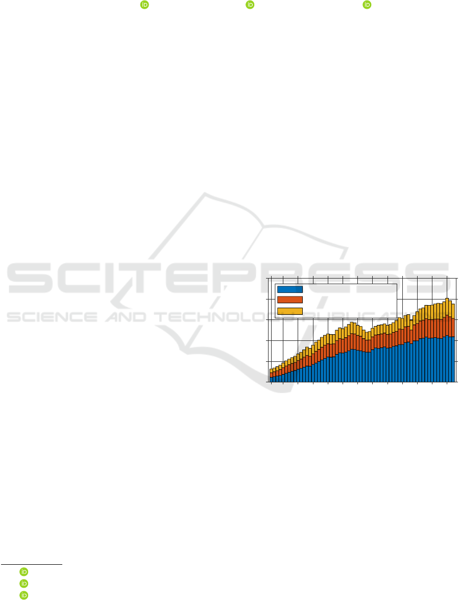
wide use of fertilizers increasing to 195.38 million
tons in 2021 (Figure 1), 90% of fertilization costs are
attributed to the fertilizer itself. In the past, farm-
1961 1965 1970 1975 1980 1985 1990 1995 2000 2005 2010 2015 2020
0
50
100
150
200
250
Consumption in million metric tons
Nitrogen (N)
Phosphorus pentoxide (P
2
O
5
)
Potassium oxide (K
2
O)
Figure 1: Global consumption of agricultural fertilizer from
1961 to 2022, by nutrient (in million metric tons). Data
from: International Fertilizer Industry Association (ifas-
tat.org).
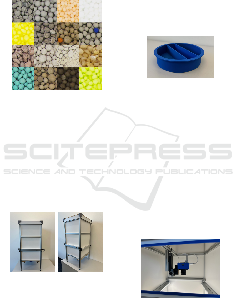
ers had limited fertilizer options, but today they must
deal with thousands of products (Figure 2), including
blends and biofertilizers. Fertilizer types can be dis-
tinguished by physical characteristics such as density,
volume, and granularity.
Rather than relying on a variety of sensors to ex-
tract these characteristics, we propose a simple and
straightforward hardware setup for image aquisition,
followed by a state-of-the-art CV-ML pipeline. This
pipeline is built using YOLO11 (Redmon et al., 2015)
and Segment Anything 2 (Ravi et al., 2024). Models
are trained using only a small set of handcrafted sam-
Lippel, J., Bihlmeier, R. and Stuhlsatz, A.
A Computer Vision Approach to Fertilizer Detection and Classification.
DOI: 10.5220/0013189300003912
Paper published under CC license (CC BY-NC-ND 4.0)
In Proceedings of the 20th International Joint Conference on Computer Vision, Imaging and Computer Graphics Theory and Applications (VISIGRAPP 2025) - Volume 3: VISAPP, pages
563-569
ISBN: 978-989-758-728-3; ISSN: 2184-4321
Proceedings Copyright © 2025 by SCITEPRESS – Science and Technology Publications, Lda.
563

ples in an active learning-based approach.
Figure 2: Cuttings from images of the 16 fertilizers used in
the project.
2 SYSTEM DESIGN
The motivation for our system design is an indus-
trial requirement to develop a cost-effective method
for testing and detecting fertilizers with as little man-
power needed as possible. This also includes the de-
velopment of a testing device for the controlled and
standardized recording of photos. The presented sub-
system is part of a bigger research project aiming to
create an application that enables fertilizer samples to
be analyzed and, if necessary, measured under labo-
ratory conditions.
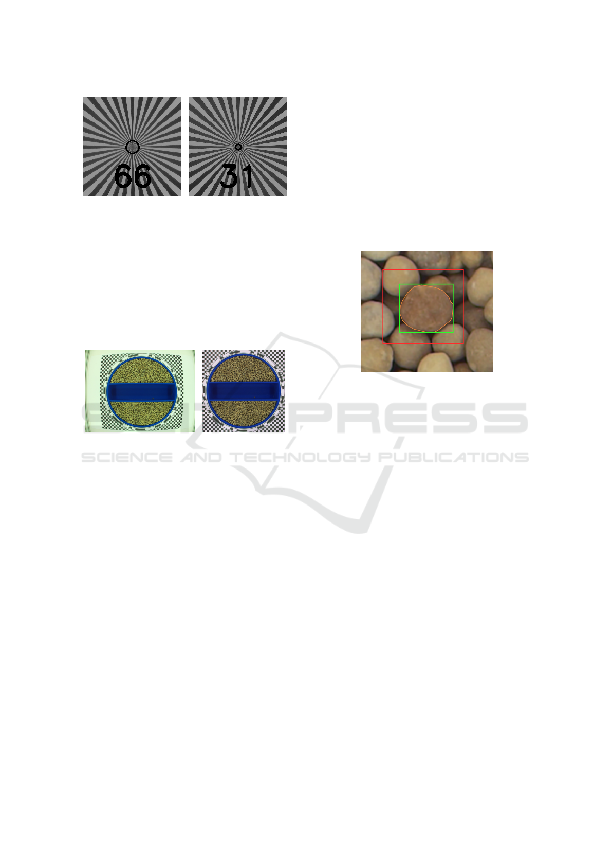
2.1 Hardware Setup
(a) Front view (b) Side view
Figure 3: Imaging box.
A controlled environment is essential for obtaining
reproducible results, particularly in CV applications
where consistent image capture is key. To achieve
this, we designed a small, portable, and cost-effective
imaging box. The box is constructed with an alu-
minum frame, white cardboard side panels, and a
wooden lid, which together provide a nearly light-
tight seal to minimize external light interference (Fig-
ures 3(a),3(b)). The bottom is sealed with a wooden
plate that includes a cutout for a sample cup (Figure
4). With a radius of 87.5 mm, the sample cup is 3D-
Figure 4: Sample cup.
printed from PLA and divided into three sections: two
crescent-shaped sections and one nearly rectangular
section. The division can be adjusted depending on
the specific needs. This setup allows for capturing im-
ages of multiple specimens simultaneously, speeding
up the image acquisition process. In our specific ap-
plication it enables to take images of multiple fillings
of the same sample at once. The plate also contains
a mounting bracket to securely hold the sample cup
in place, while allowing it to be rotated if needed. To
illuminate the interior of the box, we installed four
independently controllable LED light bars, each pro-
viding 485 lumens with a color temperature of 4000K
(Figure 6). The light bars emit diffuse light, which,
in combination with the white cardboard side panels,
ensure even illumination throughout the imaging box.
Additionally, the angle of the lights can be adjusted
as needed to achieve optimal lighting conditions. For
image capture, we used a Raspberry Pi HQ Camera
Module equipped with the default 6mm lens, con-
nected to a Raspberry Pi 4. The camera is securely
mounted on an aluminum extrusion, which is fixed to
the frame of the box to ensure stability and consistent
positioning (Figure 5).
Figure 5: Camera closeup.
A checkerboard pattern was printed on the inside
VISAPP 2025 - 20th International Conference on Computer Vision Theory and Applications
564

of the bottom plate to evaluate the effect of the undis-
tortion algorithm that will be applied (cf. Figure 9(b)).
The cutout in the bottom plate (with a radius of 91.5
mm) allows the camera to capture images of the sam-
ple cup and its content, which is mounted below the
box.
Figure 6: Light bar.
2.2 Software Solution for Imaging
Creating a fast, easy-to-use and expandable software
solution for capturing images was a key goal of this
project. For this purpose, we developed a modular,
all-in-one solution that can be easily expanded and
customized to meet the specific needs of any project.
The software is written in Python and consists of
two main components: an image acquisition module
running on the Raspberry Pi, and a control module
that manages the Raspberry Pi’s actions. This con-
trol module runs on a local computer, which we re-
fer to as the control computer. Additionally, the con-
trol computer receives the captured images wirelessly
from the Raspberry Pi via MQTT (using Mosquitto
(Light, 2017)) for further image processing. We
chose MQTT because it is a lightweight, open-source
protocol that is easy to set up and use (MQTT.org,
2024). It allows us to send the images to multiple
destinations (e.g., the control computer and a backup
server) simultaneously via an MQTT broker running
on the Raspberry Pi. Our implementation includes
the following key features: adjusting the camera fo-
cus (as the lens does not have autofocus), capturing
images and wirelessly transmitting them to the con-
trol computer, performing white balance adjustments,
and undistorting images to correct for lens distortion.
Configuring the software for both the imaging box
and the control computer is straightforwardly done
using a simple configuation file on each device. The
configuration file contains all the necessary parame-
ters for the software to run, including the IP address
of the MQTT broker, the camera’s exposure time(s)
and gain(s), as well as the names of the specimens to
be captured. One of the key challenges we encoun-
tered was finding a reliable solution for adjusting the
camera’s focus. Initially, using a live feed from the
Raspberry Pi on the control computer to fine-tune the
focus through manual inspection proved ineffective,
as the images often appeared blurry due to imprecise
adjustments. To overcome this, we developed a soft-
ware module that uses a Siemens star (similar to ISO
12233:2017) and basic CV techniques to quantify the
focus adjustment. A Siemens star is a test pattern
used for calibrating the sharpness of a camera lens
(Figure 7). Adjusting the camera’s focus affects the
Figure 7: Siemens star.
size of the gray area in the center of the star — the
smaller the area, the sharper the image. In our setup,
the star is placed on the bottom of the imaging box at
the same distance from the camera as the sample cup,
ensuring an accurate calibration of the focus. The
process starts by capturing a single image of the star.
Then a simple template matching algorithm based on
2D correlation coefficiants identifies the center of the
star which is used for further calculations. Next, the
camera captures a continuous stream of images and a
Canny Edge Detection algorithm (Canny, 1986) is ap-
plied to detect the edges of the star. In the gray area,
edge detection fails to find edges, allowing us to cal-
culate the radius of this area using the center of the
star. This radius is displayed on the screen to sup-
port the user when setting the focus to minimize the
gray area for optimal sharpness (Figure 8). Once the
focus is optimized, the corresponding value is saved
with a timestamp for documentation. To ensure con-
sistent colors in the images, we disabled the camera’s
automatic white balance and implemented a custom
white balance correction method. First, we captured
an image of a surface that we defined as white (e.g.
a piece of paper). The average color of this image is
then compared to true white (RGB: 255, 255, 255),
and the resulting factor is used to correct the white
balance for all subsequent images. In a final step, we
used checkerboard patterns of a fixed size to apply
A Computer Vision Approach to Fertilizer Detection and Classification
565

(a) Bad sharpness calibra-
tion
(b) Good sharpness calibra-
tion
Figure 8: Screenshots taken from the GUI for the sharpness
calibration process.
an undistortion algorithm (Zhang, 2000), (Heikkila
and Silven, 1997) for the correction of lens distortion.
To ensure optimal corrections, three images of the
checkerboard patterns at different orientations were
used for undistortion. Figure 9 (a) and (b) show the
raw image and the undistorted, centered, and white-
balance-corrected image, respectively.
(a) raw image (b) Undistorted, cen-
tered and white balance
corrected image
Figure 9: Data preprocessing.
Afterwards to this pre-processing, we applied a
simple detector for the circular markings on the edge
of the sample cup. This gives us a circular cropped
image. The two circular segments with the fertilizer
samples are then cut out and rotated into a uniform po-
sition as shown in Figure 11. Those cropped images
are later used for training and testing the ML-Pipeline.
3 CV-ML PIPELINE
For a robust detection and classification of fertilizer
outlines and types, we propose a processing pipeline
utilizing state-of-the-art tools, trained in an active
learning approach. First, we trained a classifier to dis-
tinguish grains from other objects in the image. To
accomplish this, a few grains of each fertilizer are la-
beled by hand in the images captured with the imag-
ing box. These markers are defined to be rectangu-
lar bounding boxes around individual grains. With
this small number of samples a first weak detector
model is trained which in turn is used to process more
images resulting in a bunch of new bounding boxes.
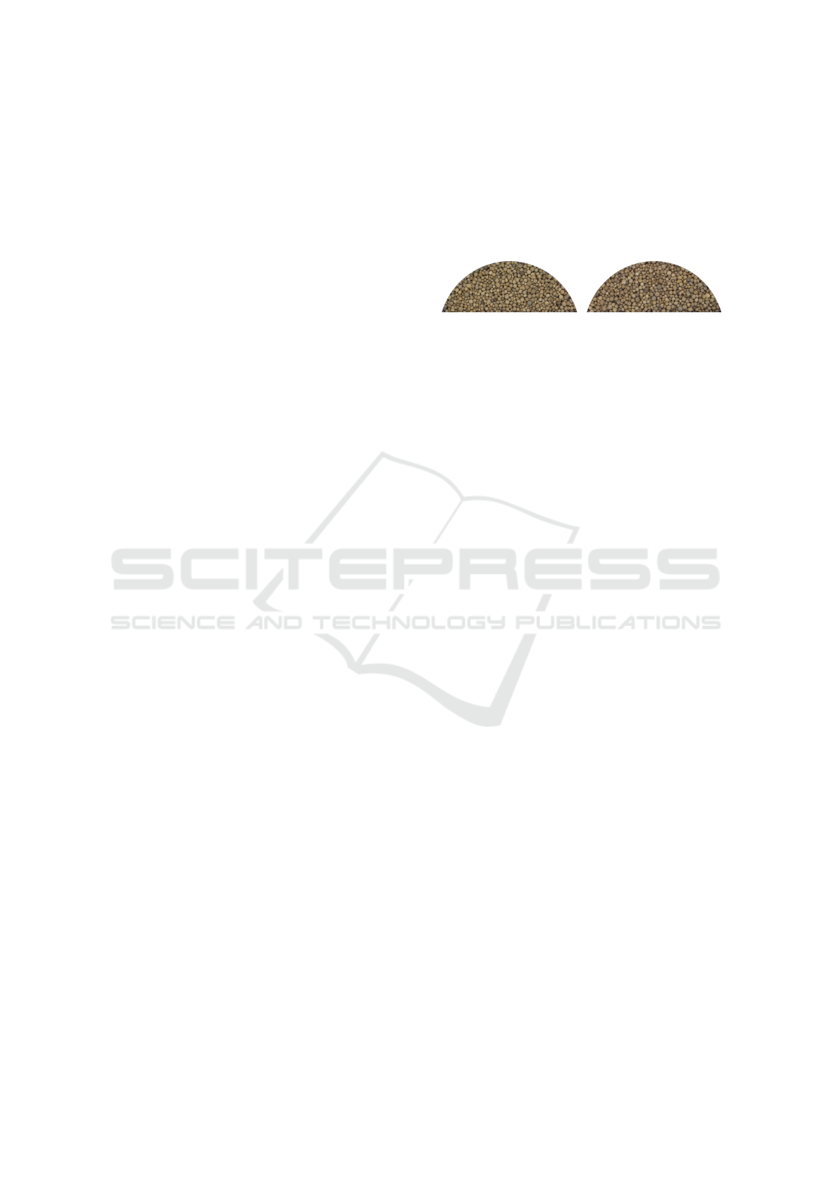
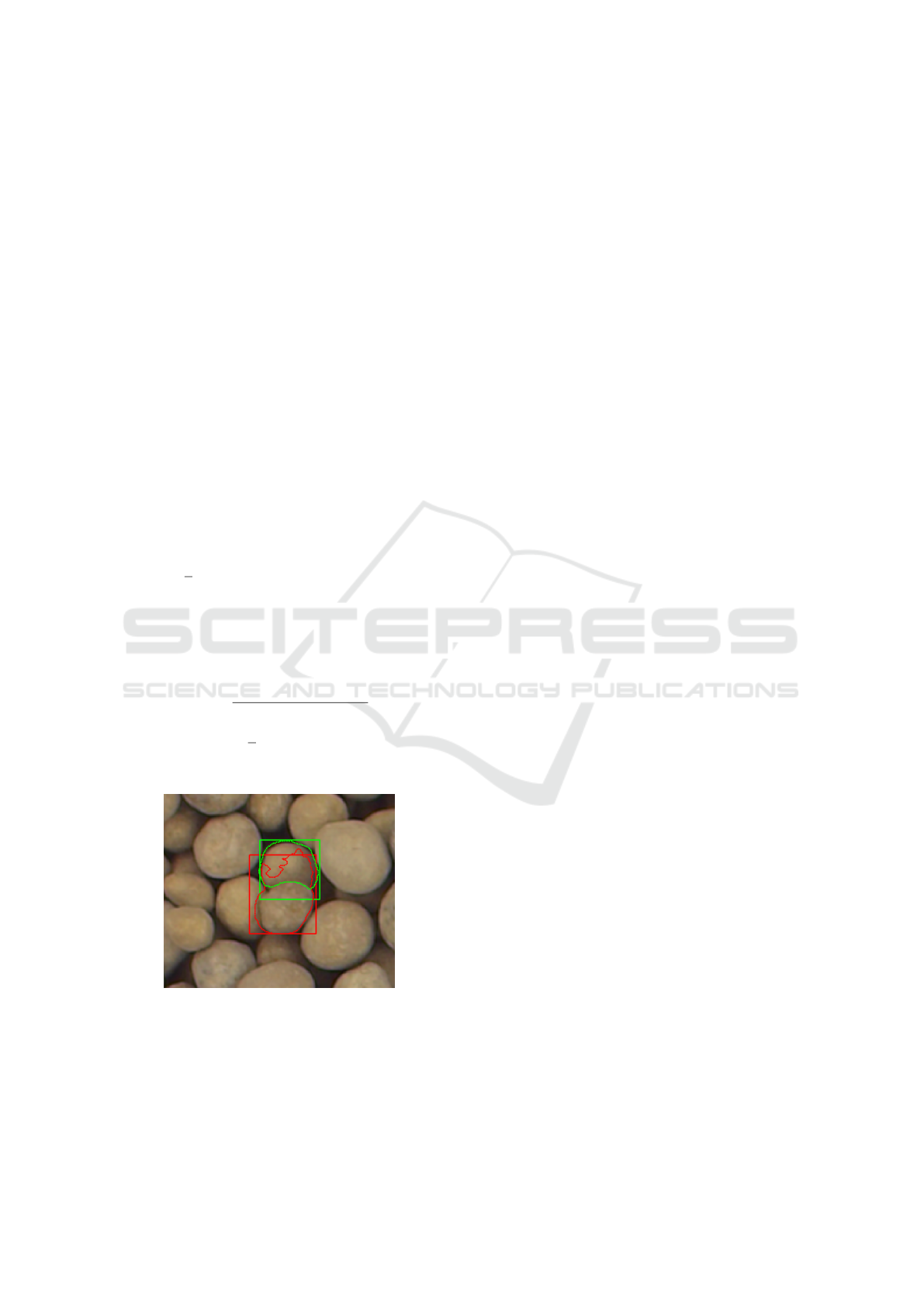
Because of the weakness of the detector the bound-
ing boxes are inaccurate (cf. red rectangle in Figure
10). To improve the accuracy, the detected bounding
boxes are fed into a segmentation system with zero-
shot generalization to unfamiliar objects and images.
This results in a contour that encloses the grain ex-
actly within any weak bounding box. Then the extent
of the contour is used to shrink the weak bounding
box to an accurate bounding box (cf. green rectangle
in Figure 10).
Figure 10: Illustration of the box refining process. Red rect-
angle: shows the best guess of the first weak detector. Or-
ange outline: shows the result of the zero-shot segmentation
system. Green rectangle: new box defined by the limits of
the outline.
In a next step, these new bounding boxes together
with the available category (i.e. type of fertilizer) are
used to train an improved grain detector and a clas-
sifier for the type of fertilizer. Afterwards, we ap-
plied this model to detect grains in the provided unla-
beled images. Although these steps could be repeated
many times to improve the accuracy, in our applica-
tion one step already yields a refined model detecting
very accurate bounding boxes with high classification
accuracy from a small number of handlabeled sam-
ples. However, to calculate shape specific parameters
of each fertilizer grain, we run the zero-shot segmen-
tation system once again to extract outlines. To elim-
inate overlapping detections, a few post-processing
steps are carried out.
In summary, the processing steps of our pipeline are
as follows:
1. train a weak detector and classifier for fertilizer
grains using a few hand-labled images
2. extract outlines and refine bounding boxes
3. train a refined detector and classifier for the type
of fertilizer
4. use refined model to detect and classify fertilizer
grains of unlabeld images
5. extract outlines and post-process detections
VISAPP 2025 - 20th International Conference on Computer Vision Theory and Applications
566

In the following sections, we describe these steps in
more detail.
3.1 YOLO and SegmentAnything
YOLO11 is the newest version of the well known
object detection model. It is capable of real-time
detection and can be easily adapted to different tasks.
YOLO11 provides pretrained models for different
tasks (e.g. detection, segmentation, pose estimation,
etc.) which can be easily finetuned with custom data.
In this paper, only the model for object detection
from YOLO11 is used, which provides bounding
boxes, a class label as well as a confidence score for
each detected object of an image.
Because YOLO11 resamples the input images depen-
dent on their resolution, we use SAHI (Slicing Aided
Hyper Inference) (Akyon et al., 2022) for slicing the
original image into overlapping slices of constant
resolution. Afterwards, multiple detections whithin
each image are combined using a non-maximum-
suppression algorithm.
For the segmentation we use the Segment Any-
thing Model 2 (SAM2). SAM2 is a segmentation sys-
tem with zero-shot generalization that provides robust
results with some known context. This context is ei-
ther one or more known points inside (or outside) of
the object to be segmented or else a bounding box ap-
proximating the outer bounds of the object. The latter
is used in the context of this paper.
As (Alif and Hussain, 2024) shown in their compre-
hensive review, YOLO is very well suited for applica-
tions in an agricultural context. We therefore decided
in favor of the use of YOLO as detector and subse-
quent SAM2 for obtaining the contours, as these two
tools meet the industrial requirements described at the
beginning: They are easy to use and powerful enough
to perform grain detection and segmentation without
the need for extensive manual labeling.
3.2 Training
We conducted a total of 3 photo sessions for taking
images of fertilizers as sample dataset.
Session 1. A total of 44 photos of 22 classes
were taken, resulting in 88 images of circle segments.
Thus, each image shows either the lower or the upper
part of the filled sample cup (Figures 11(a) and 11(b)).
The 22 classes consist of 16 different types of fertiliz-
ers (cf. Figure 2), 5 different types of spherical airsoft
bullets (exactly 5.95 mm of diameter) and one type of
plastic granulate. The six non-fertilizer classes, along
with their known parameters (e.g. diameter, round-
ness) have been added to improve monitoring our re-
sults. We split the dataset into two halves: 44 images,
i.e. exactly two of each class, showing only the upper
part of the sample cup are used in all training pro-
cesses. The remaining 44 images of the lower part of
the sample cup are used only once for testing.
(a) ROI lower part (b) ROI upper part
Figure 11: Relevant regions of the filled sample cup,
cropped and rotated to a uniformly position.
Session 2. A total of 46 photos of 23 classes were
taken, resulting in 92 images of circle segments. In
addition to session 1, we have added an additional
class: small PVC tube segments in various colors
with a length of 5 mm, an outer diameter of 5 mm
and an inner diameter of 2.5 mm. We also replaced
the camera and lens. They are the same models, but
in contrast to session 1, the camera in session 2 does
not have an infrared cut filter. This resulted in images
with a different color spectrum. As in session 1, we
again divided the data set in half and used images of
the upper part of the sample cup for training and the
lower part exclusively for testing.
Session 3. The same setup as in session 2, but
this time we readjusted the focus, aperture and camera
position and took all images of non-fertilizer classes.
We then readjusted the focus, aperture and camera po-
sition and took all fertilizer images. This procedure
enabled to achieve slight variations in the setup and
simulate a more realistic real-world application. The
images taken in this way are used exclusively for test-
ing.
To train our first simple and thus weak grain detec-
tor we manually labeled 604 grains with fitted bound-
ing boxes around each grain (approximately 20-30
boxes per class, 10-15 per image) using only the im-
ages taken in session 1. The original image size is
907x2435 pixels with smaller grains being only about
30 pixels wide. In general, detecting small structures
in large images is challenging for many detectors.
To improve the training results we therefore sliced
all images to 640x640 pixels beforehand. The sliced
images were additionally modified by distorting all
non-labeled regions of the slice by simply swapping
pixel positions around randomly. This is done to pre-
vent the model from seeing unlabeled data during the
training process, as this would lead to a bad training
performance. The weak grain detector is trained for
A Computer Vision Approach to Fertilizer Detection and Classification
567

a specific task: distinguishing grains from other ob-
jects in the image. We finetuned the YOLO11 model
yolo11x with 100 epochs of training using one class
and all other parameters in default mode.
As already shown in Figure 10 the resulting
bounding boxes of the first simple detector are still
weak due to the limited amount of training data. In the
following we use this simple detector to generate fur-
ther training data. The procedure is always as follows:
As the images have a very high resolution and the ob-
jects to be detected are relatively small, the YOLO
detector with SAHI and a confidence threshold of
0.5 is used. This process produced numerous (weak)
bounding boxes across the training images, which
the SAM2 model sam2-hiera-large uses as input to
find the outline of one grain per bounding box. The
low confidence score of the YOLO11+SAHI detec-
tor sometimes results in many bounding boxes which
may lead to faulty segmentations, as shown in Figure
12. The rectangles are the bounding boxes found by
the detector. The dashed lines are corresponding out-
lines of the SAM2 model. Green colored lines indi-
cate a higher score compared to the red colored detec-
tions. To compare the detections a mean score is cal-
culated by S = 0.5(S
YOLO
+ S
SAM2
) where S
YOLO
is
the resulting confidence score of the YOLO11+SAHI
detector and S
SAM2
the score of the SAM2 detection
respectively. To find the faulty detections, we calcu-
late the Intersection over Minimum (IoM) for all pairs
of detections A and B with
IoM =
area(A ∪B)
min(area(A), area(B))
.
If for a pair of contours IoM > 0.3 is true, the contour
with the lower score S is discarded (shown in red in
Figure 12).
Figure 12: Example of postprocessing contours. Rectan-
gles: detected grains. Dotted curves: contours found by
SAM2. Green: kept. Red: discarded.
The new bounding boxes are defined by the ex-
tend of the contours. This procedure of boosting the
amount of training samples results in a huge amount
of new training samples.
In order to be able to assess the performance, two
different experimental setups were carried out.
Training Setup 1. Only the training data from im-
age acquisition session 1 is used. These are 44 images
from 22 classes. Boosting leads to approx. 25000 new
training labels. The yolo11x model is fine-tuned again
with 100 epochs of training, but now including all 22
classes for detection.
Training Setup 2. In addition to the 44 images
from 22 classes from acquisition session 1, the train-
ing data from acquisition session 2 is now also used.
This is an additional 45 images from 23 classes. The
additional class (the colored tube segments) was also
automatically labeled with the simple grain detector.
This worked well and emphesizes the good perfor-
mance of the stack of YOLO and SAM2.
3.3 Results & Outlook
For the test of the model obtained from training setup
1 all of the 44 test images of image acquisition session
1 are used as input and processed as follows:
• detect bounding boxes with the fully trained 22
class YOLO11+SAHI detector
• find segmentations inside of each bounding box
with the SAM2 model
• postprocess detections to discard bad detections
(cf. section 3.2)
This procedure yields exactly 24692 detected con-
tours of which 24691 are correctly classified, i.e. a
test accuracy of 99.996%. As shown in Figure 13, the
results are very accurate.
These are really good results, but could be influ-
enced by the uniform arrangement in session 1. Only
images from a single shooting situation were used,
which might have made recognition an easy task.
For training setup 2 two different tests were con-
ducted following the same procedure as before: Here,
the test data from image acquisition sessions 1 and 2
were used. This resulted in exactly 47679 detected
contours, of which 100% are identified as the correct
class. This is another outstanding result, which could
again be attributed to the similarity of the test data to
the training data. To counteract this, another test run
was carried out with the data from recording session
3. As well as in the previous test results, no data from
this session was ever used for training. But beyond
that, the shots from this session represent a configura-
tion of focus, aperture and exact camera position not
previously used in any training situation. For this test
images the upper as well as the lower part of the sam-
ple cup are used. The test on this data leads to exactly
VISAPP 2025 - 20th International Conference on Computer Vision Theory and Applications
568

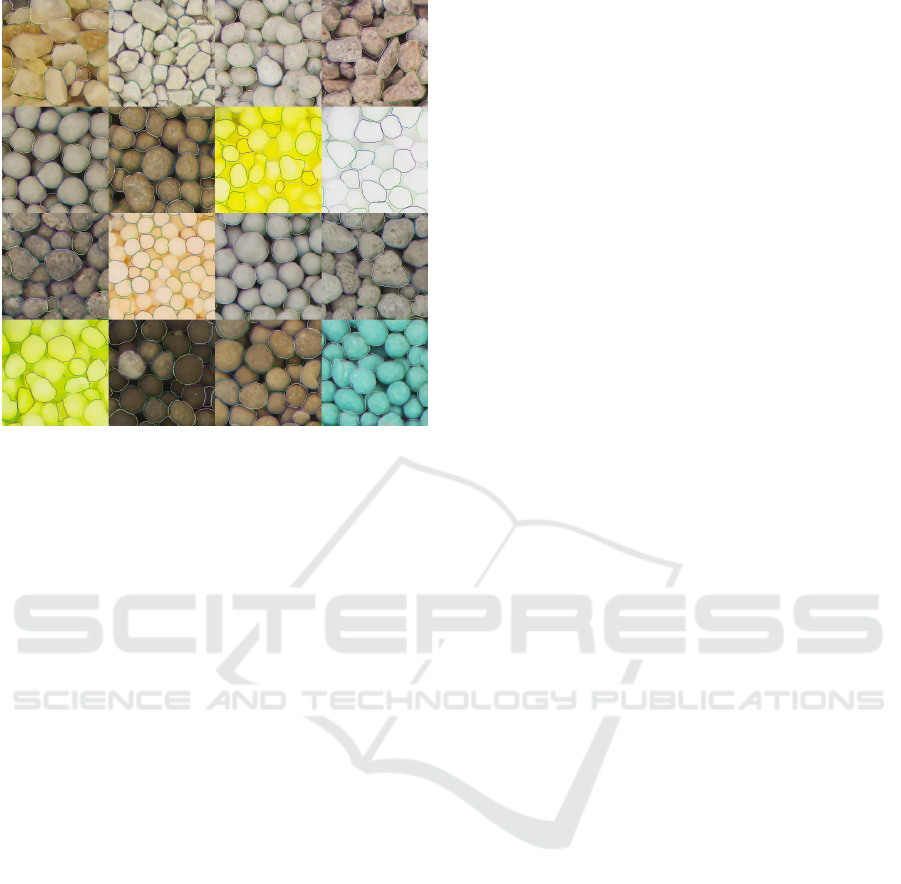
Figure 13: Cuttings from images of the 16 fertilizers used
in the project.
47736 contours of which 47693 were correctly rec-
ognized yielding a recognition rate of 99.901%. Pro-
vided the photo box presented in this paper is used in
similar situations, this result can be considered reli-
able for a real-world application too.
Future work will now involve further analysis of
the resulting contours in terms of size, shape and sta-
tistical distribution of grain sizes.
4 CONCLUSIONS
We presented a CV-ML pipeline composed of state-
of-the-art tools, namely YOLO11 and SAM2, for the
detection and classification of fertilizer grains. Using
a Raspberry Pi HQ Camera mounted in a purpose-
built imaging box with a simple diffuse light source,
the system setup is fairly simple. Training the detec-
tor and classifier in an active learning approach from
only a few manually labeled images resulted in a test
accuracy of 99.996%, despite the simplicity of our
proposed setup. Although our focus was the classi-
fication of fertilizer as part of a bigger system, our
proposed setup and pipeline can also serve as a tem-
plate for other similar applications.
ACKNOWLEDGEMENTS
This work is supported by the Federal Ministry
for Economic Affairs and Climate Action, ZIM,
KK5243405LF3.
REFERENCES
Adhinata, F. D., Wahyono, and Sumiharto, R. (2024). A
comprehensive survey on weed and crop classification
using machine learning and deep learning. Artificial
Intelligence in Agriculture, 13:45–63.
Akyon, F. C., Onur Altinuc, S., and Temizel, A. (2022).
Slicing aided hyper inference and fine-tuning for small
object detection. In 2022 IEEE International Con-
ference on Image Processing (ICIP), pages 966–970.
IEEE.
Alif, M. A. R. and Hussain, M. (2024). Yolov1 to yolov10:
A comprehensive review of yolo variants and their ap-
plication in the agricultural domain.
Canny, J. (1986). A computational approach to edge de-
tection. IEEE Transactions on Pattern Analysis and
Machine Intelligence, PAMI-8(6):679–698.
Dhanya, V. G., Subeesh, A., Kushwaha, N. L., Vish-
wakarma, D. K., Nagesh Kumar, T., Ritika, G., and
Singh, A. N. (2022). Deep learning based computer
vision approaches for smart agricultural applications.
Artificial Intelligence in Agriculture, 6:211–229.
Ghazal, S., Munir, A., and Qureshi, W. S. (2024). Com-
puter vision in smart agriculture and precision farm-
ing: Techniques and applications. Artificial Intelli-
gence in Agriculture, 13:64–83.
Heikkila, J. and Silven, O. (1997). A four-step camera cal-
ibration procedure with implicit image correction. In
Proceedings of IEEE Computer Society Conference
on Computer Vision and Pattern Recognition, pages
1106–1112. IEEE Comput. Soc.
Light, R. A. (2017). Mosquitto: server and client imple-
mentation of the mqtt protocol. The Journal of Open
Source Software, 2(13):265.
MQTT.org (2024). Mqtt: The standard for iot messaging.
Ravi, N., Gabeur, V., Hu, Y.-T., Hu, R., Ryali, C., Ma,
T., Khedr, H., R
¨
adle, R., Rolland, C., Gustafson, L.,
Mintun, E., Pan, J., Alwala, K. V., Carion, N., Wu,
C.-Y., Girshick, R., Doll
´
ar, P., and Feichtenhofer, C.
(2024). Sam 2: Segment anything in images and
videos. arXiv preprint arXiv:2408.00714.
Redmon, J., Divvala, S., Girshick, R., and Farhadi, A.
(2015). You only look once: Unified, real-time ob-
ject detection.
Sarkar, C., Gupta, D., Gupta, U., and Hazarika, B. B.
(2023). Leaf disease detection using machine learning
and deep learning: Review and challenges. Applied
Soft Computing, 145:110534.
Xie, C., Cang, Y., Lou, X., Xiao, H., Xu, X., Li, X., and
Zhou, W. (2024). A novel approach based on a modi-
fied mask r-cnn for the weight prediction of live pigs.
Artificial Intelligence in Agriculture, 12:19–28.
Zhang, Z. (2000). A flexible new technique for camera cal-
ibration. IEEE Transactions on Pattern Analysis and
Machine Intelligence, 22(11):1330–1334.
A Computer Vision Approach to Fertilizer Detection and Classification
569