Estimation of Hydrodynamic Dispersion Coefficient Under Saturated

and Unsaturated Conditions

Ziyi Jia

1,* a

, Hiroaki Terasaki

, Min Wang

, Jiehui Ren

and Wen Cheng

Graduate School of Engineering, University of Fukui, Fukui, 910-8507, Japan

Institute of Water Resources and Hydro-Electric Engineering, Xi'an University of Technology, Xi'an 710048, China

Keywords: Soil Salinization, Hydrodynamic Dispersion Coefficient, Dispersivity.

Abstract: In the study of soil salinization, the hydrodynamic dispersion coefficient is an important parameter for solute

transport. However, dispersion coefficients for soils require a great deal of time and effort, especially for silts

and clays, which can be complicated and prolonged to measure. In this study, the hydrodynamic dispersion

coefficients of silt and clay were determined by laboratory experiments and numerical analysis under different

saturation states. By comparing with the conventional method, the applicability of proposed method of to

quickly obtaining the unsaturated dispersion coefficient was verified. Additionally, by investigating the

relationship between the hydrodynamic dispersion coefficient and the soil pore water velocity, the empirical

formula of the soil hydrodynamic dispersion coefficient obtained.

1 INTRODUCTION

Soil salinization has become a common concern in

countries around the world. About 8.7 percent of the

world's land is threatened by salinization, and this

number continues to rise (FAO, 2021). China is one

of the countries with serious salinization and wide

distribution, mainly distributed in arid, semi-arid,

and coastal areas. In order to remove salinity from

soil, it is important to understand the transport

process of solutes in soil, which has been well

demonstrated in many research fields. The

hydrodynamic dispersion coefficient (D) is an

important parameter for controlling soil solute

transport. The D plays a crucial role in the simulation

and optimization of solute flux and subsequent

desalination methods.

For the measurement method of unsaturated D,

the traditional soil column method has a good effect

on sand, but it is time-consuming and labor-intensive.

In contrast, centrifugation method is fast, but the

equipment is expensive. The past developed suction

https://orcid.org/0000-0003-3688-2634

https://orcid.org/0000-0003-0087-8473

https://orcid.org/0000-0003-3110-266X

https://orcid.org/0000-0003-4491-5782

https://orcid.org/0000-0002-7231-7635

method can also be used to measure the dispersion

coefficient of sand. Although relatively cheap, it

takes a long time to reach a steady state, and the flow

needs to be adjusted. Also, due to the high cost and

time-consuming study of clay, silt, and loam, most of

the past studies have focused on the determination of

sand, highly permeable soils. In this paper, a

simplified quasi-steady-state suction method is

proposed to measure the unsaturated D of silty and

clay soils. Also, the D under the saturated state was

measured. In addition, by collecting the dispersion

coefficients of different types of soil in various

references, an empirical formula was obtained that

can be used to estimate the hydrodynamic dispersion

coefficient from the soil pore water velocity.

236

Jia, Z., Terasaki, H., Wang, M., Ren, J., Cheng and W.

Estimation of Hydrodynamic Dispersion Coefﬁcient Under Saturated and Unsaturated Conditions.

DOI: 10.5220/0013628200004671

In Proceedings of the 7th International Conference on Environmental Science and Civil Engineering (ICESCE 2024), pages 236-240

ISBN: 978-989-758-764-1; ISSN: 3051-701X

2 METHOD

2.1 Hydrodynamic Dispersion

Coefficient

Solute transport can be measured using the following

convective–dispersive equation:

∂

(1)

where C is the salt concentration (kg/m

); θ is the

volumetric water content (m

); t is the elapsed

time (s), z is position or depth (m); and Q is the solute

flux (kg/(m

·s)), which can be defined as the sum of

convective and hydrodynamic dispersive fluxes:

DqCQ

∂

−=

(2)

where q is the Darcy flow velocity (m/s), and D is the

hydrodynamic dispersion coefficient (m

/s), which is

expressed as the sum of molecular diffusion

coefficient (D

) and the mechanical dispersion

coefficient (D

D=D

+ D

(3)

In this study, the value of D

was set to 1.65 × 10

/s (Castillo et al., 1993). D

is represented by

=λv

(4)

where λ is the dispersivity (m), v is the average pore

water velocity (m/s), and α is generally equal to 1.

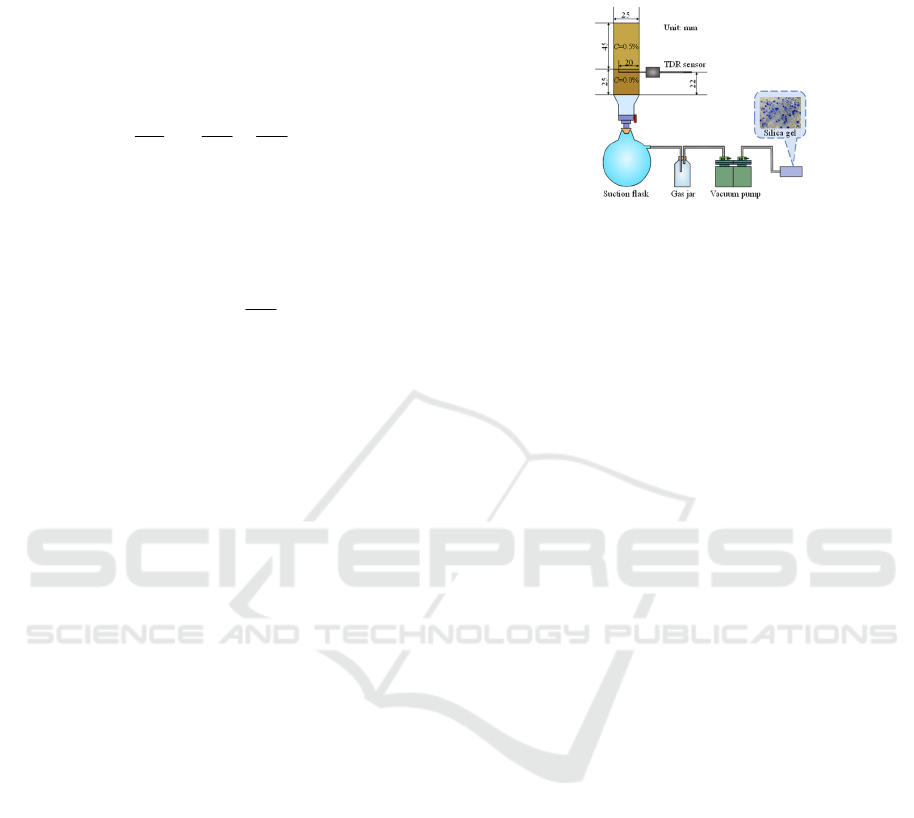
2.2 Experimental Design

2.2.1 Experiment for Unsaturated Soils

Three experimental cases using fluvo-aquic soil (a

silty soil collected from Jiangsu, China) and kaolin

clay soil were considered. The experimental setup is

shown in

Figure

1. The inner diameter of the soil

column was 25 mm, and the height was 70 mm,

which was divided into two layers. A TDR sensor

(TRIME-MUX6) was inserted near the surface of the

lower column to measure the variation in salinity.

Water suction was achieved using a vacuum pump

(DA60-D). The suction flask, gas jar, and a small

column attached at the end (filled with silica gel)

were used to collect water and water vapor. The

following experimental steps were followed: (1)

uniformly mix the soil with fresh water, and fill in

the lower soil column to a certain θ value; likewise,

fill in the upper soil column with soil mixed with

saline water (C = 0.5%) to same θ value; (2) start

water suction using the vacuum pump; (3) measure

the drainage water mass using electrical balance, and

monitor the output of the TDR sensor. To investigate

the quasi-steady-state condition, both the upper and

lower soil columns were mixed with fresh water, and

a preliminary test was conducted before the

experiment.

Figure 1: Experimental setup.

2.2.2 Experiment for Saturated Soils

Five experimental cases using fluvo-aquic soil and

Tohoku paddy soil (collected from Natori, Japan)

were considered. As shown in

Figure

2, the

experimental apparatus comprises a soil column

made of vinyl chloride, with an inner diameter of

0.107 m, pump (WP1000, Welco Co., Ltd), water

tank, funnel, electronic balance (PB4002-S, Mettler

Toledo Co., Ltd), Four-electrode salinity sensor, and

data logger (CR1000, Campbell Scientific, Inc.). The

depths of the sensors from the soil surface were 110

mm, 190 mm, 270 mm, and 350 mm. The experiment

was conducted by adopting the following procedure:

(1) The air-dried soil was screened and evenly filled

into the soil column (bulk density of 1.6 g/cm

); (2)

Kept the head of the water tank constant and

continuously supplied the fresh water from bottom of

the column to attain saturation by capillary; (3) After

saturation, the NaCl solution with C of 10 kg/m

supplied from top of the column and kept the water

level constantly; (4) Changes in the electrical

conductivity (EC) value of the sensor were observed;

(5) When the EC value of the bottom sensor was

constant, the experiment was terminated.

Estimation of Hydrodynamic Dispersion Coefﬁcient Under Saturated and Unsaturated Conditions

237

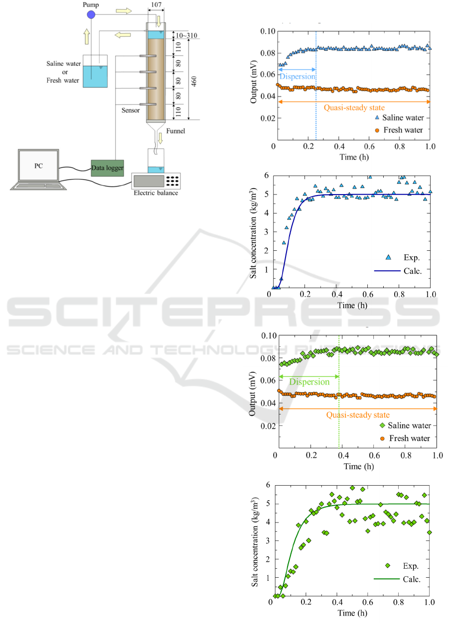
Figure 2: Experimental equipment (Unit: mm).

3 RESULTS AND DISCUSSION

3.1 Hydrodynamic Dispersion

Coefficient of Unsaturated Soil

Figure

3 shows the time variation in the output values

of the TDR sensor and salt concentration in Case1–3.

Cases 1 and 2 correspond to fluvo-aquic soil at two

flow rates. Case 3 corresponds to kaolin clay soil. No

significant changes in the TDR sensor output values

were observed in the freshwater test until 1.0 h after

the start of the experiment, which is considered a

quasi-steady state. In contrast, the TDR sensor output

value in the saline water experiment increased for

approximately 0.25 h, after which it showed a

constant value. Further, θ, C, and the TDR sensor

output obtained from the preliminary test revealed

that the salinity at the sensor position reached 0.5%

after 0.25 h.

The pore water velocity was calculated from the

time variation in the drainage mass during the quasi-

steady-state condition. The v values of the fluvo-

aquic soil were approximately 4.45 × 10

-6

m/s and

3.93 × 10

-6

m/s. The salt concentration variation

curve was obtained by converting the sensor output

value, and the dispersion coefficients were

determined by fitting the breakthrough curve for the

experimental and calculated values. As can be seen

from the breakthrough curve in Figure 3, the

calculated and experimental values have good fitness.

The D values of the fluvo-aquic soil were

approximately 2.50 × 10

-9

/s and 5.00 × 10

-9

/s,

and that of kaolin clay was 1.25 × 10

-9

/s.

Noticeably, the simplified suction method proposed

in this study yields quick results.

a)Case1– Fluvo-aquic soil

ICESCE 2024 - The International Conference on Environmental Science and Civil Engineering

238

)Case2– Fluvo-aquic soil

c)Case3–

aolin clay

Figure 3: Time variation of sensor output and breakthrough

curve of Case1–3.

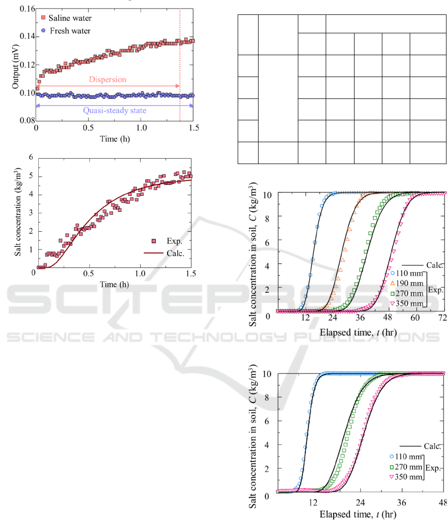
3.2 Hydrodynamic Dispersion

Coefficient of Saturated Soil

Case1–4 of fluvo-aquic soil and Case 5 of Tohoku

paddy soil determined their corresponding D at

different v as shown in Table 1. Figure 4 shows the

breakthrough curve of Case 3 and Case 5 under the

average value of 8.04×10

-7

m/s (v), by fitting the

experimental and calculated values. It can be seen

that the C changes with respect to time and space.

After adding the NaCl solution, C increased

gradually until it approached 10 kg/m

of the C.

Calculated results showed sound agreement. Due to

the scale dependency of D (Moradi et al., 2020), the

values calculated separately for each sensor from top

to bottom.

Table 1: Dispersion coefficient of each sensor at different

pore water velocity in Case1–5.

No. Soil type

D of different depth (m

/s)

(m/s)

110

190

270

350 mm

Case

Fluvo-

aquic soil

3.18E-

3.50E-

3.50E-09

Case

1.61E-

9.50E-

1.00E-

1.00E-09

Case

8.19E-

4.50E-

5.40E-

5.50E-

3.50E-09

Case

1.23E-

3.50E-

3.80E-

6.00E-

5.50E-09

Case

Tohoku

addy soil

1.77E-

7.00E-

1.80E-

2.30E-08

a)Case 3

)Case 5

Figure 4: Breakthrough curve of the saturated soil.

3.3 The Relationship between D and v

As the D of each type of soil is different, and the

measurement is complicated, the D of different types

Estimation of Hydrodynamic Dispersion Coefﬁcient Under Saturated and Unsaturated Conditions

239

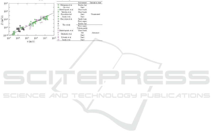
of soil in past studies are collected and summarized

in Figure 5. The relationship between the D and v

obtained in this experiment and those in the

references (Shikanuma et al., 2003; Kobashi et al.,

2004; Cho et al., 1981; Matsubayashi et al., 1997;

Taikoku et al., 1997; Kinoshita et al., 2003; Sasaki et

al., 1986; Shao et al., 2002; Takahashi et al., 2005).

The experimental values obtained in this study

generally conformed to the D-v liner line, which is

represented by:

D = 0.0095v

1.15

(5)

where the value of dispersivity is approximately

0.0095 m, and α is approximately equal to 1.15.

Figure 5: Relationship between D and v in saturated and

unsaturated soil.

4 CONCLUSIONS

In this study, the hydrodynamic dispersion

coefficients of fluvo-aquic soil and kaolin clay under

unsaturated state and fluvo-aquic soil and Tohoku

paddy soil under saturated state were investigated.

Proposed simplified suction method in this study

yields quicker results than the conventional methods.

Additionally, by collecting the different types of soil

in past studies and combing the values in this study,

the dispersivity of different saturation conditions

were measured at 0.0095 m. Therefore, when the soil

dispersion coefficient cannot be experimentally

measured under limited conditions, it can be

calculated using the dispersivity obtained in this

study when the soil pore water velocity is known.

However, the measurements are relatively few. In the

future, we will accumulate experimental data and

compare that with data from other measurement

methods to verify its accuracy.

REFERENCES

FAO, 2021. World map of salt-affected soils launched at

virtual conference.

Castillo, R., Garza, C., 1993. Temperature dependence of

the mutual diffusion coefficients in aqueous solutions

of alkali metal chlorides[J]. International Journal of

Thermophysics, 14(6): 1145–1152.

Moradi, G., Mehdinejadiani, G., 2020. An experimental

study on scale dependency of fractional dispersion

coefficient[J]. Arabian Journal of Geosciences,

13(11), 409.

Shikanuma, Y., Izawa, J., Kusakabe, O., 2003. Advective

diffusion of pollutants in clay soil using drum

centrifuge[J]. Japanese Geotechnical Society, 38:

2345–2346.

Kobashi, H., Miki, H., Hirayama, M., Hishiya, T.,

Yamamoto, H., Ohkita, Y., 2004. The determination of

longitudinal dispersivity in predicting the influence of

ground contamination[J]. Japan Society of Civil

Engineers, 764(3): 53–67.

Cho, T., Tanaka, A., Kodani, Y., 1981. A new method of

determining the dispersion coefficient of salt in soil[J].

Bull. Sand Dune Research, 20: 11–16.

Matsubayashi, U., Devkota, L.P., Takagi, F., 1997.

Characteristics of the dispersion coefficient in miscible

displacement through a glass beads medium[J].

Journal of Hydrology, 192: 51–64.

Taikoku, T., Suganuma, M., Matsubayashi, U., Takagi, F.,

1997. A study on the advection and diffusion

characteristics in a heterogeneous porous medium[C].

Japan Society of Civil Engineers Annual Meeting, Ⅱ–

185.

Kinoshita, K., Hayashi, S., Oka, T., 2003. Understanding

dispersion phenomena in unsaturated permeation flow

based on vertical column experiments[J]. Japan

Society of Civil Engineers, 2: 71–72.

Sasaki, Y., Sato, K., Fukuhara, T., 1986. Experimental

study on diffusion and dispersion coefficients of

solutes in unsaturated seepage flow[C]. Japan Society

of Civil Engineers Annual Meeting, Ⅱ–91.

Shao, A., Liu, G., Yang, J., 2002. In-lab determination of

soil hydrodynamic dispersion coefficient[J]. Acta

Pedological Sinica, 39: 184–189.

Takahashi, N., Nakata, M., Yamamoto, Y., 2005. Study on

hydrodynamic dispersion and absorption

characteristics of soil. Sumitomo Mitsui Construction

Technology Research Report, 3: 65–69.

ICESCE 2024 - The International Conference on Environmental Science and Civil Engineering

240